
Shape from Texture
Proceedings of the Ninth International Joint Conference on Artificial Intelligence. Perception. Pages 926-930.
© 1985 International Joint Conferences on Artificial Intelligence
Abstract
Measurements on image texture interpreted under an app rox im ate perspective image model can be used with an iterative eonstraint propagation algorithrn to determine sur faee o ri entation. An extension of the ideas allows their robust applieation to natural images of textured planes. The t ee hniques are demonstrated on synthetie and natural images.
- Aho. A.V., Hopcroft, J.E. and Ullman, J.D., The Design and Analysis of Campwer Algorithms, Addison-Wesley Publishing Co., Reading. MA ., 1974.
- Aloimonos, J. and Chou, P., "Detection of surface orientation and motion from texture." forthcoming Technical Report, Dept. of Computer Science. Univ. of Rochester.
- Bandyopadhyay, A.. "lnteresting poims. disparities and correspondence," Proceedings, DARPA Image Understanding Workshop, Ocrober 1984.
- Bajcsy, R. and Lieberman, L.. "Texture gradients as a depth cue." Camp. Graphics and Image Processing S, 1976, 52-67.
- Ballard, D.H. and Brown, C.M., Computer Vision, Prentice-Hall, lnc., Englewood Cliffs, NJ, 1982.
- Gibson, J.J., The Perception of the Visual World, Houghton Miffin, Boston, 1950.
- Horn, B.K.P., "Understanding image intensities," Artificia/ I ntel/igence 8, (2), 1977. 201-23 L
- lkeuchi, K., "Shape from regular patterns," Artificial lntelligence 22, 1984, 49-75.
- J. Aliomonos and M. Swain 931
- lkeuchi, K. and Horn, B.K.P .. "Numerical shape from shading and occluding boundaries," Artificia/ lntelligence 17. 1981. 141• 184.
- Kanade. T., "Recovery of the three dimensional shape of an object from a single view," CMU•CS• 79-153. Dept. of Comp. Science, Carnegie-Mellon Univ., 1979.
- Kender, J.R .. "Shape from texture: an aggregation transform that maps a dass of textures into surface orientation," Proceedings, IJCAI, 1980, 475-480.
- Kender, J.R, "Shape from texture: A computational paradigm," Proceedings, DARPA Image Understanding Workshop, April 1979, 79-84.
- Marr, D. and Hildreth, H .. "A theory of edge detection." Al Memo 518, MIT, 1979.
- Ohta, Y., Maenobu, K., and Sakai, T., "Obtaining surface orientation of from texels under perspective projection," Proceedings, IJCAI, 1980, 746•751.
- Witkin, A.. "Recovering surface shape and oricntation from texture," Artificia/ lntelligence 17, 1981. 1 7•45.
References were extracted automatically from the PDF and may contain errors.
Full text extracted automatically from the PDF; figures, tables and equations may differ. The PDF is the version of record.
Abstract
Measurements on image texture interpreted under an approximate perspective image model can be used with an iterative eonstraint propagation algorithrn to determine surfaee orientation. An extension of the ideas allows their robust applieation to natural images of textured planes. The teehniques are demonstrated on synthetie and natural images.
L lntroduction
The reeovery of 3-D (shape) information from a two dimensional image is an important task in image understanding. "Shape from ... " algorithms exist for intensity, motion, contour, and texture. This work extends work on Shape from Texture. The shape from texture problern has been studied extensively. Gibson (1950) first proposed the texture density gradient as the primary basis of surfaee pereeption by humans. Following Gibson's ideas, Bajesy and Lieberman (1976) tried a heuristie use of the two dimensional Fourier speetrum to detect the gradient.
To formalize the shape from texture problern requires a model for the image Formation system. Up to now three kinds of projeetions have been used: Orthographie, perspeetive and spherieal projection. Kender (1980), Kanade (1979) and Witkin (1981) studied the problern under Orthographie projeetion, and Kender (1980) and Ohta (1981) address the problern under perspective projeetion. lkeuehi (1984) used spherieal projection. In his work the texture elements had to be known and symmetrical.
Our algorithm determines surfaee orientation from the apparent distortion of patterns on the image, provided that:
- (l) The surfaee in view is smooth and is covered with uniformly repeated texture elements. All the texture elements on the surfaee are identical. These texture elements we call texels. The shape of the texels is of no importanee for our theory.
- Eaeh texture element is assumed to lie on a plane (i.e. we assume that the surface in view is loeally planar). This means that the size of the texels on the surfaee has to be small eompared with a change of surface orientation . there.
Shape from texture
lohn Aloimonos and Michael J. Swain Department ofComputer Science The University of Rochester Rochester, N.Y. 14627
(3) The scene texture is imaged under an approximation to perspeetive projection similar to that of Ohta (1981). This projection preserves important perspective distortions but is computationally tractable.
Under the above assumptions, we develop a new gradient map that will enable us to define a "textural reflectance function.". Our theory is very similar to earlier work on Shape from Shading (Horn, 1977; lkeuchi, 1981), with the image intensity at a point replaced with the are<J of the image texel at that point.
2. Mathematical preliminaries
In this section we define a way to approximate the distortion of a texel under perspective projection by a 2-D affine transformation.
2.1 Approximation of the perspective projection by a 2-D affine transformation
Let a coordinate system OXYZ be fixed with respect to the camera, with the -z axis pointing along the optical axis, and 0 the nodal point of the eye (center of the lens). The image plane is assumed to be perpendicular to the Z axis at the point (0,0,-1), (i.e. focal length = 1).
Under perspective projection, a point of the object surface is projected onto the image plane by a projecting ray defined by that point and the eenter of the lens.
Our approximation is dorre by dividing the projection process into two steps. (See figure 1). Consider a textured surface S in the world and a texel T on the surface, lying in a loeal plane Q with orientation given by the surface gradients (p,q). Consider also a plane y, parallel to the image plane and just in front of the surface S. The plan~ y has distance ß from the origin, (i.e. its equation is -z = ß).
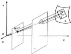
--- 6 --- The steps of the projection process of the texel T onto the image plane are as follows:
- The surface texel is projected onto the plane y. This projection is performed parallel to the ray OG, where G is the mass center of the texel T. (Thus the image of the mass center of the texel is on the projected mass center of the texel, and the projection is parallel to the direction (A,B,-1) where (A,B) is the image of the mass center of the texel T).
(2) The image on the plane y is projected perspectively onto the image plane. Since the plane y is parallel to the image plane, this perspective transformation is just a reduction by a factor of 1/ß.
Step 1 skews the image to account for foreshortening, and step 2 scales the image in a location-depth dependent manner, as does perspective. The combined process is an affine transformation.
To represent the original pattern of the surface texel, we use an (a,b,c) coordinate system, with its origin at the mass center of the texel and the (a,b) plane identical to the plane Q. To represent the pattern of the image texel, we use an (a',b',c') coordinate system, with its origin the point (A,B,-1), i.e. the mass center of the image texel, and the axes a',b',c' parallel to the axes X,Y,Z respectively. Then the transformation from (a,b) to (a',b') with the two step projection process of previous section is given by the affine transformation.
It is clear that this transformation is the relation between two 2-D patterns, one in the 3-D space and the other its image on the image plane. We now use the above affine transformation to develop the desired constraint.
2.2 The constraint
The determinant of the matrix of an affine transformation is equal to the ratio of the areas of the two patterns before and after the transformation. Specifically, if Sw is the area of a world texel that lies on a plane with gradient (p,q) and s 1 is the area of its image that has mass center (A,B), then we have:
Equation (1) relates the area of a world texel s W· its gradient (p,q), the area s 1 of its image and its mass center (A,B). If we call the quantity s 1 "textural intensity," and the quantity Swlß 2 "textural albedo," then equation (1) is very similar to the image irradiance equation
where I is the intensity, (p,q) the gradient of the surface point whose image has intensity I, ;\ is the albedo at that point and (A,B,l) the direction of the light source (Horn, 1977: lkeuchi, 1981).
Thus equation (1) can be used to recover surface orientation, using methods that have been discovered for the solution of the shape from shading problern (lkeuchi, 1981).
2.3 A gradient map
Equation (1) of the previous section can be written as :
where I is the texturai intensity, i.e. the area of an 1mage texel with mass center (A,B), and
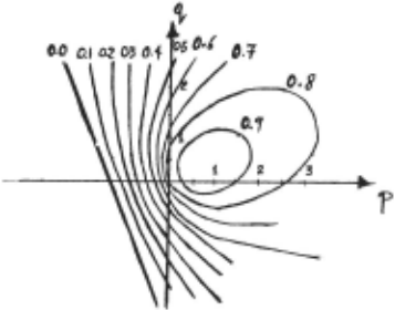
with ;\ the texturai aibedo, i.e. the quantity Swlß2, and (p,q) the gradient of the plane on which the world texel lies. The function R(p,q) we call textural reflectance. I f we fix the albedo ;\, and the position (A,B) of the texel on the image, then equation (2) can be represented conveniently as a series of contours of constant textural intensity. Figure 2 illustrates such a simple textural retlectance map.
2.4 Recovering the textural albedo
We use equation (2) of the previous section to recover the locai surface orientation. No matter what method we use we must know the textural albedo ;\=Swlß 2 .
We cannot know ß from a static monocular view; neither can we know Sw in general. But it turns out that we can compute approximately the ratio Swlß2, i.e. the textural aibedo ;\.
Consider three neighboring image texels T 1 , T 2 and T 3 with areas 1 1 , 1 2 and 1 3 and we suppose that the world texels whose images are the texels T 1 , T 2 and T 3 lie on the same plane with gradient (p,q). Then the following equations arise:
where n = (p,q,l)/ J1 +p 2 + q 2 and si = (-Ai, -Bi, 1) for i= 1,2,3 and (Ab Bi) the mass center of texel Ti. Eliminating the textural albedo t.. from the equations (3), (4) and (5) we get:
for some constant k that makes n a unit vector, where
and provided that [s 1 ,s2,s 3 1 ~ 0, i.e. the vectors s 1 , s 2 ; s 3 are not coplanar (linearly dependent).
The result of equation (7) is approximate due to the hypothesis that three neighboring texels lie on the same plane. But, if we perform this process in all the triples of neighboring points, and we take the average value for the albedo, then the result is highly improved. At the same time, we can get an approximate value for the surface normals at all the texels in the image (equation (6)). Then we can use these initial approximations to start the iterative algorithrn that will be introduced in the next section.
2.5 Another way to recover the albedo
Following Ohta et al. (1980) and assuming local planarity, i.e. three neighboring texels belang to the same plane which we call Q, we have that:
where 1 1 · f2 are the distances from two texels to the vanighing line of the plane Q along the line joining the two texels and s 1 , 5 2 are the areas of the two texels in the image. Since [f 1 - !21 is just the distance between the two texels in the image and it is known, a point on the vanishing line may be determined. With a third texel, two points may be determined, which give the equation of the vanishing line. Since the equation of the vanishing line of the plane Q is px + qy = 1, the orientation of the plane Q can be determined, and from that an approximation of the textural albedo is found.
3. Additional constraints and propagation of the constraints
In this section we introduce the smoothness constraint (!keuchi, 1981) and we present an iterative algorithm of the same flavour as the one introduced by lkeuchi.
3.1 An iterative propagation algorithm
We have already proved that every distortion value (image texel area) for a specific image position corresponds to a contour in the gradient space (See section 3.4). So, the problern has infinite solutions (is "ill-posed") and this is the reason that we introduce the smoothness assumption (a "regularization condition"). A smoothness constraint can be used to reduce the locus of possible orientations to a unique orientation, through an iterative algorithm.
Trying to develop a global error function that should be minimized in order to give the desired value, we measure the departure from smoothness and the error in the textural reflectance equation (equation 2). The error in smoothness we measure (after lkeuchi, 1981) as follows:
where Pu and qiJ derrote the orientation at the surface point whose image is the point (ij). The error in the textural reflectance equation, can be given by :
where f .. is the distortion value (texel area) at the point I,] (ij) and R the textural reflectance.
An acceptable solution should minimize the sum of the error tenns in all the grid nodes. lf Eis such a global error function, then
and the factor w gives a weight to the errors in the textural gradient map relative to the "distance" from smoothness. To minimize E, we differentiate with respect to P· . and q . . and setting the resulting derivatives to zero 1,] l,p and rearranging the equations we obtain:
where pa . . and qa . . are the average values of p and q 1,] I,] around the point (ij) respectively. The above equations suggest an adjustment of p and q in the direction of the gradient of the textural reflectance function, by an amount that is proportional to the error in the textural reflectance equation (equation 2). So it is natural to use the following iterative rule for the estimation of the p and q everywhere in the image:
In the above equations the partial derivatives of the textural reflectance are evaluated on the values of p and q of the n-th iteration. Finally, to avoid numerical instabilities we modify the above formulas to the following form (lkeuchi & Horn, 1981):
R(pi,jqi) is a function on a four-dimensional space, unlike the R(p,q) of orthographic Shape from Shading. The shading R(p,q) can be determined empirically, but the textural reflectance R(pi.J·qi) is an analytic, geometrical entity arising from imaging geometry, and thus only the global constant (texture) albedo varies from texture to texture and scene to scene.
4. Experiments
The algoritl-Jm was tested on artificial images of a plane, cytinder and sphere. There are four distinct steps into which the program may be broken down:
- Location of texels
- Minimum triangulation of the texel centers
- Calculation of initial orientations and textural albedo.
4) Iterative process.
In 1), the connected regions in the image are detected. Their centers of gravity are taken to be the locations of the texels. Their size is recorded and the texels which are in the boundary are marked (Ballard & Brown, 1982). In 2), the points denoting the centers of the texels are triangulated so that the sum of the length of the lines is minimum (Aho, Hopcroft & Ullman). In 3), the initial orientations were calculated using the method in Section 3.6. The estimate of A. was calculated from the local orientation with the lowest value of p and q. Due to · curvature of the surface, convex objects tend to give an overestimate of A. while concave objects tend to give an underestimate. These errors are minimized when the surface of the object is most nearly perpendicular to the image plane. The algorithm is quite insensitive to initial orientations given to texels whose orientations were allowed to vary through the iterative process. Boundary texels were not allowed to change. The error in calculating their values was the predominant factor in influencing the total error. The iterative process took under 10 iterations. The process always converged for our synthetic images. The final error values were
fractional error
| plane | negligible |
|---|---|
| sphere | .005 |
| cylinder | .015 |
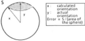
The errors in the above table denote the average percent error at each texel. The error at each texel was taken to be
where <p = solid angle subtended by rotating the calculated orientation about the actual orientation. Figure 3 gives a pictorial description of the error at each texel.
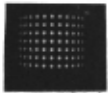
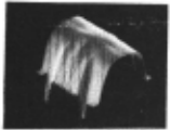
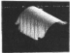
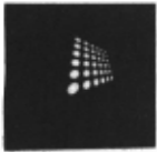
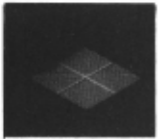
Finally, azimuthat equidistant coordinates (AEC) were used through the iterative process instead of the gradient space p and q, since AEC change linearly with change in orientation. Figure 4 shows the image of a sphere which is covered with a repeated pattern, Figure 5 shows the reconstructed sphere using the algorithms of Sections 3.5 and 3.6, · and Figure 6 shows the reconstructed sphere after the relaxation. Figures 7, 8, and 9 and 10, 11, and 12 show the analogaus pictures for a cylinder and plane respecti vely.
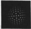
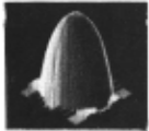
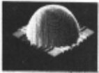
Figure 5
5. An extension to natural images
In natural images, the assumption that the world surface is covered with the same texels is not very realistic. This section refers to recent work by Aloimonos and Chou (1985) on shape from the images of textured planes, based on the uniform density assumption under strong segmentation (identification of texels) and weak segmentation (edge finding). Consider a world plane - z = px + qy + c, and the plane y passing through the center of mass of a small area s of the world plane. I f we consider an area s 1 in the image, then in order to find the area in the world plane whose projection is s 1 . we must multiply the area s 1 with the factor
where (A,B) is the center of gravity of the image area s 1 .
5.1 Exploiting the uniform density assumption
The uniform density assumption states that if K, I\ are any two regions in the world plane and they contain K 1 and K 2 texels respectively, then Ktfarea(K) = K/area(/\). So considering any two regions SJ and s2 in the image with areas s 1 and s 2 that contain K 1 and K 2 texels respectively, then under the assumption that the world texels are uniformly distributed, we have K 1 ;s 1 R 1 = K/S 2 R 2 with
and (A 1·82), (A2,B2) the centers of gravity of the image regions s 1 and s 2 respectively.
The above equation represents a line in p-q space. Any two regions in the image constrain (p,q) to Iie on a line in the gradient space. Thus, taking any two pairs of regions we can solve explicitly for p and q. (To overcome undesirable results due to errors from the digitization process and the density fluctuations of the regions, we employed a least-square-fit mechanism by considering several image pairs. A Hough transform estimation method might also be appropriate.) Figure 13 is the image of a plane parallel to the image plane, covered with random dots (texels). Figure 14 is the image of the dotted plane rotated and translated with tilt = 135° and slant = 30°. Our program, based on the scheme described above, recovered tilt = 134.4° and slant = 29.75°.
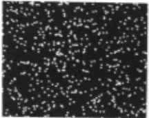
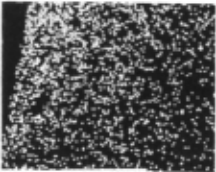
Figure 14
5.2 Solving the problern with a weaker segmentation
In the previous section a method was developed to recover the orientation of a textured plane from its image, based on the assumption of uniform texel density; by uniform density, we mean that the number of texels per unit area of the world plane is the same. Application of this method to natural images did not seem to work very weil , because no good methods have been developed up to now that can identify texels in an image, and this algorithm depends critically on the number of texels per unit area. On the other hand, in the recent Iiterature
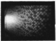
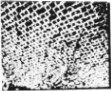
(Bandyopadhyay, 1984; Ballard & Brown, 1982; Marr, 1979) there are several methods for the . computation of partial boundaries of the texels (edges) at every point in a textured image. Let us redefine density to be the total length of the texel boundaries per unit area. The uniform density assumption states that this density is the same everywhere in the world plane. This assumption is not far from the previous one and seems to be true for a !arge subset of natural images, in cantrast with Witkin's isotropy assumption, which does not seem to hold true for many natural images. Aloimonos & Chou (1985) describe a method that finds the orientation of the world plane under the new assumption and below we describe expriments based on that method. Figure 15 presents the image of a plane parallel to the image plane, covered with random line segments. Figure 16 presents the image of this plane rotated with tilt = 135° and slant = 30·. The program recovered tilt = 133.77· and slant = 30.40·. Figure 17 presents the image of a plane (parallel to the image plane) covered with randomly generated small circles. Figure 18 presents the image of this plane rotated with tilt = 135· and slant = 30·. The program recoverd tilt = 135.54· and slant = 29.77· . The natural images used were first preprocessed to find the boundaries of texels (edges) by applying the modified Frei-Chen operators introduced by Bandopadhyay (1984). Figure 19 shows the photograph of a textured floor with slant::::::: 45· and tilt::::::: - 108·. Figure 20 shows the edges after the proprocessing. The algorithm produced slant = 45.87" and tilt = -109.43·. Finally, Figure 21 shows the photograph of a part of a grass field with slant = 60· and tilt = o·. Figure 22 shows the images of its edges after the preprocessing. The program recovered slant = 63.057" and tilt = -1.076·.
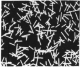
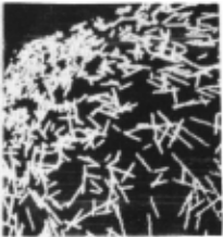
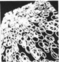
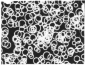
Figure 18
·
Aloimonos and Chou (1985) present a theoretical analysis of the error introduced by the affine approximation to the perspective projection.
Conclusion
In this paper we gave a method for "shape from texture" computation that extends results in the literature. Our algorithm can work in a richer domain than already published methods. For reasons involving the cosine foreshortening law, the result here is similar to the original Shape from Shading constraint applied to lambertian surfaces. We believe that this may have some important implications, since for example the same hardware may be used for shape recognition, regardless of whether we use shading or texture. Finally, an extension of the algorithm to a form that works weil for many natural images was presented.
@inproceedings{ijcai1985p187,
  title     = {Shape from Texture},
  author    = {Aliomonos, John and Swain, Michael J.},
  booktitle = {Proceedings of the Ninth International Joint Conference on
               Artificial Intelligence, {IJCAI-85}},
  publisher = {International Joint Conferences on Artificial Intelligence},
  editor    = {Aravind Joshi},
  pages     = {926--930},
  year      = {1985},
  note      = {Perception},
  url       = {https://ijcai.org/proceedings/1985/187},
}
TY - CPAPER TI - Shape from Texture AU - Aliomonos, John AU - Swain, Michael J. T2 - Proceedings of the Ninth International Joint Conference on Artificial Intelligence, IJCAI-85 PB - International Joint Conferences on Artificial Intelligence PY - 1985 SP - 926 EP - 930 UR - https://ijcai.org/proceedings/1985/187 ER -Copied
Machine-readable versions of this paper, for tools and AI agents:
 Welcome
 Future Conferences
 AI Journal Division
 IJCAI Proceedings
 About IJCAI
 IJCAI Awards