An Inference Technique for Integrating Knowledge from Disparate Sources

1. Single Belief Functions

We assume that a knowledge source, KS 1 , distributes a unit of belief across a set of propositions for which it has direct evidence,** in proportion to the weight of that evidence as it bears on each. This is represented by a function:

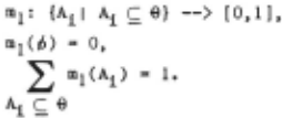
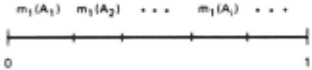
m1(Ai) represents the portion of belief that KS1 has committed exactly to proposition Ai· termed its "basic probability mass." m1 can be depicted as a partitioned unit line segment, the length of each subsegment corresponding to the mass attributed to one of its focal elements (Figure 1). Any mass assigned to a represents the residual "uncertainty" of the KS directly. That is, m 1 (a) is the mass that could not be ascribed to any smaller subset of a on the basis of the evidence at hand, but must instead be assumed to be distributed in some (unknown) manner among the propositions discerned by 9. A similar interpretation is given to mass assigned any (nonunit) set.

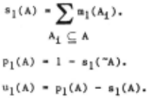
Once mass has been assigned to a set of propositions, the evidential interval can be determined directly. Support for a proposition A is the total mass ascribed to A and to its subsets; the plausibility of A is one minus the sum of the mass assigned to -A and to subsets of -A; the uncertainty of A is equal to the mass remaining, i.e., that attributed to supersets of A, including Q,

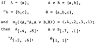
For example,

2. Composition of Mass Functions

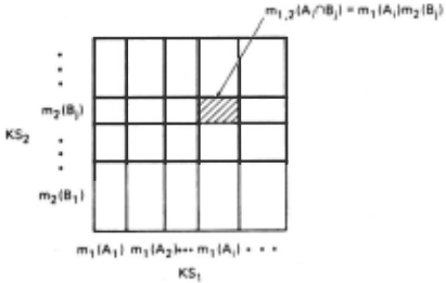
If the belief function of a second KS, KS2· is also provided, the information supplied by these KSs can be pooled by computing the "orthogonal sum;" this computation is illustrated by the unit square in Figure 2.

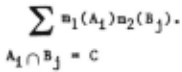
To combine the effects of KS 1 , and KS 2 , we consider the unit square as representing the combined probability mass of both KSs; KS 1 partitions the square into vertical strips corresponding to its focal elements, while KS 2 partitions it into horizontal strips that correspond to its focal elements. For example, Figure 3 shows a vertical strip that is exactly committed to Ai horizontal strip of size m2CBj) to B 1 by KS 2 · The intersection commits exactly m1(Ai)m2(Bj) to Atn Bj. of measure ml(Ai) by KS 1 , and a committed precisely of these strips the combination of Accordingly, we can compute the area commitment of each rectangle comprising the square. A given subset of 9, C, may have more than one rectangle exactly committed to it; the total mass allocated to C is This scheme is likely to commit a portion of mass to the empty set 6. Every rectangle committed to Ain Bj, where Ai n Bj · 6, results in such a commitment. The "remedy" is to discard all such rectangles, proportionally increasing (i.e., normalizing) the size of the remaining rectangles by the following multiplicative factor:

where

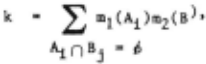
thereby restoring the total probability mass to one.

There are several points of interest with respect to Dempster's rule of combination. The operation is commutative; therefore, the order of combination is immaterial. The operation is also associative, allowing the pairwise compositions of a sequence of KSs. When two Bayesian mass functions are combined, one associating its full unit of mass with a single proposition, the resulting support and plausibility values are the expected Bayesian conditionals. Yet when only less precise information is available, it too can be exploited.

The degree of conflict between two KSs can be measured intuitively by the size of the factor k. The greater the value of k, the greater the degree of conflict between the two KSs. When k is one, the KSs are irreconcilably different and the orthogonal sum does not exist.

B. Inference Rules

In addition to a technique for pooling distinct bodies of evidence, rules are needed that allow evidential information to be translated from those propositions it bears upon directly to those it bears upon indirectly. These rules are based on the following two principles of evidential support:

• The proposition corresponding to the frame of discernment always receives full support.
• Any support committed to a proposition is thereby committed to any other proposition it implies.

From the first principle we know that s(9) ~ p(9) · 1. The second principle dictates that any support committed to a subset of the frame of discernment is thereby committed to its supersets. This follows because one proposition implies another if it is a subset of that proposition in the frame of discernment. Of the total support committed to a given proposition A, some may be committed to one or more proper subsets of A, while the rest is committed exactly to A --and to no smaller subset, i.e., m(A). If it is assumed that a knowledge source expresses itself in terms of support and plausibility estimates for a selected set of propositions from the frame of discernment, a set of inference rules allows these estimates to be translated from proposition to proposition, thereby reducing uncertainty. A sampling of these rules follows. The statements above the line in each rule allow the statement below the line to be inferred.

Ace A[0,1). A[s1(A),p1(A)) A[s2(A),p2(A)) A[s(A),p(A)), s(A) · MAX[ s1(A), s2(A) ), p(A) · MIN[ p1(A), p2(A) ), A[s(A),p(A)) -A[s(-A),p(-A)), s(-A) · p(-A) · A[s(A),p(A)) 8 [s(B),p(B)) A v 8[s(AvB),p(AvB)), - p(A), - s(A). s(AvB) a MAX[ s(A), s(B) ), p(AvB) · MIN[ 1, p(A) + p(B) ),

A v 8 [s(AvB),p(AvB)) A[s(A) ,p(A) I 8 [s(B),p(B)), s(B) ~MAX[ 0, s(AvB) - p(A) ), p(B) ~ p(AvB). A[s(A),p(A)) 8 [s(B),p(B)) A & 8 [s(A&B),p(A&B)], s(A&B) · MAX[ 0, s(A) + s(B) - 1 ), p(A&B) ~ MIN[ p(A), p(B) ), A & 8 [s(A&B),p(A&B)) A[s (A), p(A)] 8 [s(B),p(B)), s(B) · s(A&B), p(B) · MIN[ l, l + p(A&B) - s(A) ).

As can be easily shown, when propositions are known to be true or false (that is, when their corresponding belief intervals become either [0,0] or [1,1)), these rules reduce to the corresponding rules of the propositional calculus. Thus, when appropriate knowledge exists, this method will enable easy transition from a probabilistic inference computation to the· standard propositional calculus.

III EXAMPLE: MODELING A KNOWLEDGE SOURCE

As our intention has been to treat sensors as specialized KSs, in this section we shall describe an approach to modeling such a KS. We shall begin by discussing the usual parameters measured by a (hypothetical) sensor, illustrating how, for this simple example, these measurements are converted to hypotheses by the inference mechanism.

A. Sensor Measurements

We assume that collections of electromagnetic signal "emitters" deployed in various configurations comprise the situation of interest. Measurements of characteristics of the signals emitted by these devices will be used to formulate hypotheses about their identities. In the complete system, these hypotheses will interact with those derived from other KSs to create a more comprehensive picture of the situation. Let us first concern ourselves with a single KS and then show how it may be composed with other KSs.

1. Emitter Characteristics

In this example, an emitter will radiate a pulsed radar signal whose pertinent characteristics will include the carrier frequency (rf) and the pulse width (pw), which are measured directly by the receiver. For the example we assume that the emitters of interest are of types E1, E2, E3, E4, or ES. The goal of the program is to identify a signal as having originated from one of those types.

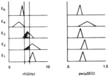
The information about the parameter values likely to be exhibited by an emitter is presented in the form of parameter distribution graphs--for example, as shown in Figure 3. These curves indicate the probability that any given emitter (of the type indicated) will have a specific parameter value; the total area under each curve is one.

A typical approach to identifying an emitter is to look up the measured parameters in a t a ble. In addition to difficulties traceable to the static nature of the table (e.g., emitter characteristics are not expected to remain stable and constant in actual operation), the technique gives little information regarding the relative likelihoods of ambiguous identifications.

2. Sensor Characteristics

A sensor (receiver) will specify a range of possible values for the measured emitter parameter, as determined by the resolution of the sensor's measurements. For example, the receiver may specify an emitter's frequency value as lying within a band of frequencies, say from 5.5 to 5.6 GHz. Similarly, other emitter parameters will also be specified as falling within a range of values.

Our previous work [1) described how sensor models were modified in the event of changing environmental conditions. In the approach des cribed here, such environmental factors will instead determine the total mass a sensor may allocate to propositions other than e. In effect, the uncertainty U of a receiver in the prevailing conditions is its minimal commitment toe (i.e., m(Q) > U), leaving only (1 - U) of the mass to be freely distributed.

B. Modeling the Operation of ~ Sensor

The modeling process begins with the determination of a frame of discernment. If the task is to determine the true value of some variable, the frame of discernment is the set of all possible values for that variable. For the problem at hand, each element of the frame of discernment consists of an emitter type paired with a feature vector representing one possible electromagnetic signature that such an emitter might exhibit. Thus, e is a subset of all of the combinations of emitter types (ET), radio frequencies (RF), and pulse widths (PW).

The key requirement of the frame of discernment is that all the propositions of interest be in correspondence with its subsets. In the current context the following propositions are some of those that might be of interest:

(The radio frequency is between 5.5 and 5.6 GHz) · {ql q ~ e and 5.5 ~ rf(q) ~ 5.6};

(The emitter is type El with pulse width between .68 and .7~o~s)

• {ql q ~ e and et(q) · El and .68 ~ pw(q) ~ .7}.

Once a frame of discernment has been determined, it can be represented as a dependency graph [5). In this formalism propositions are represented by nodes, their interrelationships by arcs. These interrelationships can be interpreted either as set-theoretic notions relative to the frame of discernment (e.g., intersection, union, inclusion, and complementation), or as logical connectives (e.g., conjunction, disjunction, implication, and negation). The appropriate subset of propositions and relationships, so represented, depends on the preferred vocabulary of discourse among the KSs. Those propositions to which the KSs tend to assign mass need to be included, along with those relationships that best describe their interdependence. Once such a dependency graph has been established, it provides an integrated framework for both the combination and extrapolation of evidential information.

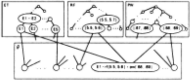
In the current context there is a subgraph for each emitter feature. At the lowest level of these subgraphs is a set of propositions representing the smallest bands into which that continuous feature has been partitioned--this partitioning being necessary within a propositional framework. These primitive bands form the basis of a hierarchy in each subgraph, relating larger bands to more primitive ones. The emitter types are similarly represented, the higher elements in the hierarchy corresponding to disjunctions of emitter types. All this is tied together by one last subgraph that relates the base elements of the hierarchies to elements of the frame of discernment, the frame of discernment consisting of the possible combinations of base elements. Figure 4 is a sketch of this dependency graph, with each node representing a proposition equal to the disjunction of those immediately below it, and the conjunction of those immediately above it.

This dependency graph contains all the information needed to determine the collective impact of several bodies of evidence on all the propositions of interest. Given several distinct bodies of evidential information extracted from the environment by several knowledge sources, repeated applications of Dempster's rule followed by repeated applications of the inference rules for support and plausibility propagation--all based on the information embodied in the dependency graph-­ results in a support and plausibility estimate for every proposition of interest [5]. There are no restrictions regarding which propositions serve as premises or conclusions. Information about radio frequency and pulse width can be used to determine the most likely types of emitters--or information about emitters and pulse width can be used to predict the expected radio frequency. Inferencing is unconstrained.

C. Simplification of the Sensor Model

In the preceding discussions, we showed how inferences could be drawn in a formal system that modeled all relevant elements of e. It is frequently inconvenient to model these elements individually. For example, too many elements may be needed to represent the resolution of any particular sensor. An obvious simplification is to compute new propositions in e as they are needed. For example, when a receiver reports a signal in a specific frequency band, propositions can then be created which assert that the signal originated from one element of a subset of possible emitter types. The exact hypotheses and their associated mass allocations are determined by comparing receiver measurements with tabulated information about the emitters.

1. Initial Mass Computations

The first step is to convert sensory measurements into a probability mass distribution over propositions. In essence, the parameter measurement range is overlaid on the curves representing distributions of emitter parameters, as shown in Figure 3. The area of the distribution curve is computed for each emitter (propositions are created only for those emitters whose parameter ranges overlap the sensor's report). A set of "basic mass numbers" is then computed by normalizing the resultant areas to bring their total area to one. This process is exactly equivalent to computing the probability of each emitter, conditioned upon the measured parameter's falling in the specified range (and assuming that only the tabulated emitter could radiate the received signal).

The uncertainty U of the receiver is accounted for through reducing each basic mass number by multiplying it by a factor equal to one minus U. This new set of mass numbers then represents the contribution of the receiver measurement to the support of the proposition.

2. Example

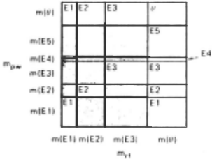
In this example we assume that there are five emitter types {E1, ··· , E5}, whose rf and pw characteristics are shown graphically in Figure 3. The receiver has reported a frequency measurement of 7.6 to 7.7 GHz and a pulse width range of .68 to .7 IJ.S· Assuming an uncertainty of .3 in the rf measurement and an uncertainty of .2 for pw, the resulting mass functions are

Combining these with Dempster's rule gives the composite mass function,

with a resulting uncertainty of 0.11. This computation is illustrated in Figure 5,in which all rectangles attributed to 6 are shaded and the remaining rectangles labeled with the proposition receiving that mass. These values convert directly to intervals on the propositions, as shown:

E 1 [.25, .36]

E 2 [.16 .27]

E3 '

E 4 [.33, .43] [.018, .13]

E 5 [ .14, .25]

This information may be readily combined with information provided by other KSs. For example, a KS that indicated a high likelihood of encountering an E1 might produce the following mass function:

which, when integrated with the receiver measurements, would result in a mass function

with an uncertainty of .06. This leads to the following relevant hypotheses:

Based on sensor data alone, the method leads to two primary hypotheses, E1!.25,.36l and E3r .33,.43)· E3 is slightly favored over E. When external evidence is brought to bear, the support for E1 becomes significantly greater than for all others (and, in fact, all others except E3 drop to very low levels of support). Any other KS that provides a mass assignment over this set of proposit ions may also be combined.

This simplification of the formal method provides the ability to integrate information quickly from a variety of sources, even in those areas where the necessary propositions have not already been extracted from e. The technique does not yet allow the propagation of evidence to arbit rarily selected propositions from the network. For exampie, it is not possible to take the structure defined for this problem and use it to determine what radio frequency values should be expect ed on the basis of pulse width data--a process easily carried out by the full representation. This is an area of current research. A related computational technique, restricted to evidence that either confirms or denies a single proposition, is also being investigated [6).

IV SUMMARY

We have briefly described an inference technique that appears to satisfy many of the requirements for reasoning in perceptual domains. In particular, the method provides the capability for (Bayesian) probabilistic reasoning when the appropriate underlying models are available (e.g., at the lowest levels of the system), (evidential) subjective reasoning when incomplete descriptions must be used (e.g., at the "middle" levels of the system), and (Boolean) logical reasoning when the truth values of propositions are true and false. This technique allows us to augment a static, incomplete model with current sensory information.

The approach provides a formal technique for updating the likelihoods of propositions in a consis tent manner. In effect, by simultaneously performing computations over a coll~ction of propos itions, the method maintains global consi stency without the problems frequently plaguing techniques that perform iterative updating by means of l ocal rules. Most importantly, besides offering an inference technique that can be used within a KS (as illustrated), the method provides a "language" for KSs to communicate with one another, as well as furnishing the means for linking disparate sources of information.

In our previous work on perceptual-reasoning systems, we evolved a number of effective generic (e.g., terrain, weather, etc.) and domain-specific (e.g., sensor) KSs. Our current research, focusing on the evidential propositional calculus as the integrating medium, aims at developing a general framework for linking these KSs together smoothly and flexibly.