
Computational Methods for a Mathematical Theory of Evidence
Proceedings of the Seventh International Joint Conference on Artificial Intelligence. Expert Systems. Pages 868-874.
© 1981 International Joint Conferences on Artificial Intelligence
Abstract
Many knowledge-based expert systems employ numerical schemes to represent evidence. rate competing hypoth · eses, and guide search through the domain's problem space. This paper has two objectives: first. to introduce one such scheme . developed by Arthur Dempster and Glen Shafer, to a wider audience: second, to present results that can reduce the compu · tation -time complexity from exponential to linear. allowing this scheme to be implemented in many more systems. In order to enjoy this reduction, some assumptions about the structure of the type of evidence represented and combined must be made . The assumption made here is that each piece of the evidence either confirms or denies a single proposition rather than a disjunction . For any domain in which the assumption is justified . the savings are available.
- J. A. Barnett, Computational Methods for a Mathematical Theory of Evidence: Part II. Forthcoming.
- James Bernoulli. Ars Conjectandi. 1713
- A. P. Dempster, "On direct probabilities," J. Roy. Statist. Soc . Ser. 8 25, 1963, 102•107.
- A. P. Dempster, "New methods for reasoning toward poste• nor distributions based on sample data," Ann . Math. Statis. 37 , 1967, 355•37<4.
- A. P. Dempster, "Upper and lower probabilities induced by a multivalued mapping," Ann. Math. Statis. 38, 1967, 325•339.
- A. P. Dempster, "Upper and lower probability inferences based on a sample from a finite univariant population ," Biometrika 54, 1967, 515•528.
- A. P. Dempster, "Upper and lower probabilities generated by a random closed interval," Ann . Math. Statis. 39, (3), 1968. 957•966.
- A. P. Dempster, "A generalization of Bayesian inference." J. Roy. Statis. Soc. Ser. 8 30. 1968, 205•247.
- A. P. Dempster, "Upper and lower probability inferences lor families of hypotheses with monotone density ratios," Ann . Math. Statis. 40, 1969, 953•969.
- R. 0 . Duda, P. E. Hart. and N. J. Nilsson , Subjective Bayesian meth:>ds for rule-based inference systems . Stanford Re • search Institute. Technical Report 124, January 1976. 87
- L. Friedman. Extended plausible inference. These proceed • ings. IJCAI
- T. Garvey. J. Lowrance. M. Fischler, An inference technique for integrating knowledge from disparate sources. These proceedings. IJCAI
- F. Hayes-Roth and V. R. Lesser. "Focus of Attention in the Hearsay• II Speech-Understanding System." in IJCAI77 . pp. 27•35, Cambridge. MA. 1977 . IJCAI
- H. E. Pople. Jr., "The formation of composite hypotheses in diagr.ostic problem solving: an exercise in synthetic reasc•ning." in Proc . Fifth International Joint Conference on Artificial Intelligence . pp. 1030-1037 , Dept. of Computer Science. Carnegie-Mellon Univ .. Pittsburgh . Pa .. 1977.
- G. Sraler, "A theory of statistical evidence." in W. L. Harper and C. A. Hooker (eds.}. Founda rions and Philosophy of Stati~• tical Theories in Physical Sciences. Reidel. 1975.
- G. Sr. a fer, A Mathematical Theory Of Evidence . Princeton University Press, Princeton , New Jersey, 1976.
- E. H. Shortliffe, Artificial Intelligence Series. Volume 2: Computer-Based Medical Consultations: MYCIN , American Elsevier. Inc .• N. Y.,. chapter IV, 1976.
- L.A. Zadeh, "Fuzzy sets," Information and ControlS, 1965. 338<i53.
References were extracted automatically from the PDF and may contain errors.
Full text extracted automatically from the PDF; figures, tables and equations may differ. The PDF is the version of record.
1. INTRODUCTION
How should knowledge-based expert systems reason? Clearly. when domain-specific idiosyncratic knowledge is available. it should be formalized and used to guide the inference process. Problems occur either when the supply of easy-to-formalize knowledge is exhausted before our systems pass the "sufficiency" test or when the complexity of representing and applying the knowledge is beyond the state of our system building technology. Unfortunately. with the current state of expert -system technology. this is the normal. not the exceptional case.
At this point . a fallback position must be selected. and if our luck holds. the resulting system exhibits behavior interesting enough to qualify as a success. Typically. a fallback position takes the form of a uniformity assumption allowing the utilization of a non· domain-specific reasoning mechanism: for example. the numer· ical evaluation procedures employed in MYCIN [17] and INTERNIST [14] . the simplified statistical approach described in [10] , and a multivalued logic in [18] . The HEARSAY-II speech understanding system [13] provides another example of a numer· ical evaluation and control mechanism-however. it is highly domain-specific.
Section 2 describes another scheme of plausible inference, one that addresses both the problem of representing numerical weights of evidence and the problem of combining evidence. The scheme was developed by Arthur Dempster [3. 4, 5, 6, 7, 8, 9] . then formulated by his student, Glen Shafer [15, 16]. in a form that is more amenable to reasoning in finite discrete domains such as those encountered by knowledge-based systems. The theory reduces to standard Bayesian reasoning when our knowledge is accurate but is more flexible in representing and dealing with ignorance and uncertainty. Section 2 is a review and introduction . Other work in this area is described in [12].
·This research is supported by the Defense Advanced Research Projects Agency under Contract No. OAHC15 72 C 0308. Views and conclusions conta ined in this report are the author"s ar.d should not be tnterpreted as representing the offtctal opin10r, or policy of DARPA. the US Government. or any person or a~ency tonnetted with them.
Section 3 notes that direct translation of this theory into an implementation is not feasible because the time complexity is exponential. However. if the type of evidence gathered has a useful structure, then the time complexity issue disappears. Section 4 proposes a particular structure that yields linear time complexity. In this structure, the problem space is partitioned in several independent ways and the. evidence is gathered within the partitions. The methodology also applies to any domain in which the individual experiments (separate components of the evidence) suppor1 either a single proposition or its negation.
Section 5 and 6 develop the necessary machinery to realize linear time computations. It is also shown that the results of experiments may vary over time, therefore the evidence need not be mono tonic. Section 7 summarizes the results and notes directions for future work in this area.
2. THE DEMPSTER-SHAFER THEORY
A theory of evidence and plausible reasoning is described in this section . It is a theory of evidence because it deals with weights of evidence and numerical degrees of support based upon evidence. Further. it contains a viewpoint on the representation of uncer tainty and ignorance. It is also a theory of plausible reasoning because it focuses on the fundamental operatron of plausible reasoning. namely the combination of evidence. The presentation and notation used here closely parallels that found in [16) .
After the formal description of how the theory represents evidence is presented in Section 2.1. an intuitive interpretation is given in Section 2.2. then a comparison is made. in Section 2.3, to the standard Bayesian model and similarities and differences noted. The rule for combining evidence. Dempster's orthogonal sum. is introduced in Section 2.4 and compared to the Bayesians' method of conditioning in Section 2.5. Finally, Section 2.6 defines the simple and separable support functions. These functions are the theory's natural representation of actual evidence.
2.1. Formulation of the Representation of Evidence
Let e be a set of propositions about the exclusive and exhaustive possibilities in a domain. For example, if we are rolling a die. e contains the six propositions of the form 'the number showing is i' where , ~ i~6 . e is called the frame of discernment and 29 is the set of all subsets of e. Elements of 2 9 · i.e .. subsets of e. are the class of general propositions in the domain; for example, the proposition ·the number showing is even ' corresponds to the set of the three elements ol e that assert the die shows either a 2, 4, or 6.
The theory deals with refinings , coarsenings, and enlargements of frames as well as families of compatible frames. However. these topics are not pursued here-the interested reader should see [16] where they are developed.
A function Bel :2e_ (0, 1] is a belief function if it satisfies Bel(0) = 0. Bel(9) = 1. and for any collection, A 1 ... An, of subsets of 9.
A belief function assigns to each subset of 9 a measure of our total belief in the proposition represented by the subset . The notation, Ill. is the cardinality of the set I.
A function m:2e-+(0,1] is called a basic probability assignment if it satisfies m(0) "0 and IIAC:e]m(A) = 1. The quantity, m(A) . is called A's basic probability number ; it represents our exact belief in the proposition represented by A. The relation between these concepts and probabilities are discussed in Section 2.3. If m is a basic probability assignment, then the function defined by
is a belief function. Further, if Bel is a belief function . then the function defined by
is a basic probability assignment. If equations (1) and (2) are composed in either order. the result is the identity transformatton . Therefore. there corresponds to each belief function one and only one basic probability assignment . Conversely. there corresponds to each basic probability assignment one and only one belief function. Hence. a belief function and a basic probability assignment convey exactly the same information.
Other measures are useful in dealing with belief functions in this theory. A function 0:2e-+[0.1] is a commonality function if there is a basic probability assignment. m. such that
for all A~9 . Further, if 0 is a commonality function , then the function defined by
is a belief function. From this belief function, the underlying basic probability assignment can be recovered using (2); if this is substit1,1ted into (3), the original 0 results. Therefore, the sets of belief functions, basic probability assignments, and commonality functions are in one·to·one correspondence and each represen· tat ion conveys the same information as any of the others.
Corresponding to each belief function are two other commonly used quantities that also carry the same information. Given a belief function Bel , the function Dou(A)" Bei(""'A). is called the doubt function and the function P* (A)= 1-Dou(A) = 1-Bei(...,A). is called the upper probability function .
For notational convenience, it is assumed that the functions Bel , m, 0, Dou, and P* are each derived from one another . If one is subscripted. then all others with the same subscript are assumed to be derived from the same underlying information.
2.2 . An Interpretation
It is useful to think of the basic probabtlity number . m(A). as the measure of a probability mass constrained to stay in A but otherwise free to move. This freedom is a way of imagining the noncommittal nature of our belief. i.e .. it represents our ignorance because we can not further subdivide our bE!Iief and restrict the movement. Using this allusion, it is possible to give intuitive interpretations to the other measures appearing in the theory.
The quantity Bei(A) = IIBC:Alm(B) is the measure of the total probabtlity mass constrained to stay somewhere in A. On the other hand. O(A) = I(A~s]m(B) is the measure of the total probability mass that can move freely to any point in A. It is now possible to understand the connotation interded in calling m the measure of our exact belief and Bel the measure of our total belief . If A~B~9 . then this is equivalent to the logical statement that A implies B. Since m(A) is part of the measure Bei(B) . but not conversely. it follows that the total belief in 8 is the sum of the exact belief in all propositions that imply 8 pitts the exact belief in B itself.
With this interpretation of Bel. it is easy to see that Dou(AJ = 1-Bei(...,A) is the measure of the probability rnass constrained to stay out of A. Therefore. P*(A) = 1-Dou(A) is the measure of the total probability mass that can move into A, though it is not necessary that it can all move to a single point, hence P*(A) = I(Ans·e~Jm(B) is immediate. It follows that P*(A)~Bei(A) be· cause the total mass that can move into A is a superset of the mass constrained to stay in A.
2.3 . Comparison with Bayesian Statistics
It is interesting to compare this and the Bayesian model. In the latter, a function p:2e-+[0,1] is a chance density function if I[aEe]P(a) · 1; and the function Ch:2e-[o, 1] is a chance function if Ch(0) = 0, Ch(9) · 1, and Ch(AUB) "Ch(A) + Ch(B) when Ana= 0 . Chance density functions and chance functions are in one-to-one correspondence and carry the same information. If Ch is a chance function. then p(a) "Ch({a)) is a chance density function; conversely. if p is a chance density function. then Ch(A) = I[aEAJP(a) is a chance function.
If pis a chance density function and we define m({a)) = p(a) for all a€9 and make m(A) · 0 elsewhere, then m is a basic probability assignment and Bei(A)" Ch(A) for all AE2e. Therefore, the class of Bayesian belief functions is a subset of the class of belief functions. Basic probability assignments are a generalization of chance density functions while belief functions assume the role of generalized chance functions.
The crucial observation is that a Bayesian belief function ties all of its probability masses to single points in 9, hence there is no freedom of motion. This follows immediately from the definition of a chance density function and its correspondence to a basic probability assignment. In this case. P* =Bel because. with no freedom of motion, the total probability mass that can move into a set is the mass constrained to stay there.
What this means in practical terms is that the user of a Bayesian belief function must somehow divide his belief among the singleton propositions. In some instances, this is easy. If we believe that a fair die shows an even number. then it seems natural to divide that belief evenly into three parts. If we don't know or don't believe the die is fair , then we are stuck.
In other words, there is trouble representing what we actually know without being forced to overcommit when we are ignorant. With the theory described here there is no problem-just let m(EVEN) measure the belief and the knowledge that is available. This is not to say that one should not use Bayesian statistics. In fact . if one has the necessary information. I know of no other proposed methodology that works as well. Nor are there any serious philosophical arguments against the use of Bayesian statistics. However, when our knowledge is not complete. as is often the case. the theory of Dempster and Shafer is an alternative to be considered.
2.4 . The Combination of Evidence
The previous sections describe belief functions. the technique for representing evidence. Here, the theory's method of combining evidence is introduced. let m 1 and m 2 be basic probability assignments on the same frame, e . and define m · m,em2. their orthogonal sum, to be m(0) · 0 and
when A~0 . The function m is a basic probability assignment if K_, ~0: if K_, "o. then m 1 em 2 does not exist and m 1 and m 2 are said to be totally or flatly contradictory. The quantity log K = Con(Bei, .Bel 2 ) is called the weight of conflict between Be.l1 and Bel 2 . This formulation is called Dempster's rule of comb1nat·on .
It is easy to show that if m 1 , m 2 , and m 3 are combinable, then m,em 2 -m 2 em, and (m,em 2 )em 3 =m,e(m 2 em 3 ). If vis the basic probability assignment such that v(e) = 1 and v(A) = 0 when A~e . then v is called the vacuous belief function and is the representation of total ignorance. The function . v. is the identity element for e . i.e., vern,= m, .
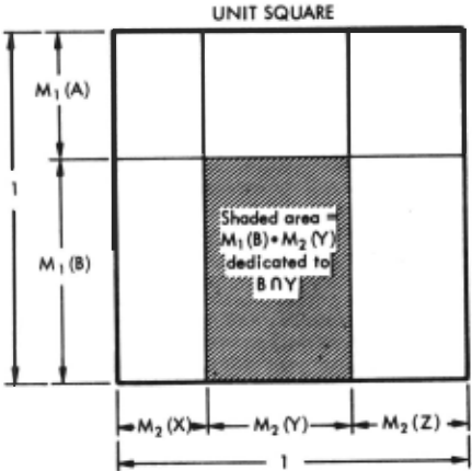
Figure 2-1 is a graphical interpretation of Dempster 's rule of combination. Assume m 1 (A) , m 1 (B)~O and m 2 (X), m 2 (Y). m 2 (Z)~O. and that m 1 and m 2 are 0 elsewhere. Then m 1 (A) + m 1 (B) .. 1 and m 2 (X) + m 2 (Y) + m 2 (Z) = 1. Therefore, the square in the figure has unit area since each side has unit length. The shaded rectangle has area m 1 (B)·m 2 (Y) and belief proper· tiona! to this measure is committed to BnY. Thus. the probability number m(BnY) is proportional to the sum of the areas of all such rectangles committed to BnY. The constant of proportionality, K. normalizes the result to compensate for the measure of belief committed to 0 . Thus. K- 1 = 0 if and only if the combined belief !unctions invest no belief in intersecting sets; this is what is meant when we say belief functions are totally contradictory.
Using the graphical interpretation, it is straightforward to write down the formula for the orthogonal sum of more than two belief functions. let m = m,e ... em 0 · then m(0) = 0 and
when A"" 0 . As above. the orthogonal sum is defined only if K- 1 ~0 and the weight of conflict is log K.
Since Bel. m. Q. Dou. and P* are in one·to-one correspondence. the notation Bel= Bel 1 eBel 2 . etc. is used in the obvious way. It is interesting to note that if 0 = 0 1 EB0 2 . then O(A) = K0 1 (A)02(A) for all A~e where A~0 .
2.5 . Comparison with Conditional Probabilities
In the Bayesian theory, the function Ch(·IBl is the conditional chance function . i.e., Ch(AIBl · Ch(AnB)/Ch(B) . is the chance that A is true given that B is true. Ch(·IBl is a chance function. A similar measure is available using Dempster's rule of combination.
Let m (B). 1 and let m 8 be 0 elsewhere. Then Bel8 is a belief functi~n that focuses all of our belief on B. Define Bei(·IBl · BeleBel . Then [16] shows that P* (AlB) · P* (AnB)/P* (B); this has the :ame form as the Bayesians' rule of conditioning. but in general. Bei(AIBl = (Bei(AU...,B)-Bei('...,B))/(1-Bei('..,B)). On the other hand , if Bel is a Bayesian belief function. then Bei(AIBl = Bei(AnB)/Bei(B) .
Thus. Dempster's rule of combination mimics the Bayesians' rule of conditioning when applied to Bayesian belief functions. It should be noted, however , that the function Bel8 is not a Bayesian belief function unless IBI = 1.
2.6. Simple and Separable Support Functions
Certain kinds of belief functions are particularly well suited for the representation of actual evidence, among them are the classes of simple and separable support functions. If there exists an F~e such that Bei(A)"s~O when F~A and A~e. Bel(e)=1 . and Bei(A) = 0 when F gA. then Bel is a simple support function , F is called the locus of Bel. and sis called Bel 's degree of support .
The vacuous belief function is a simple support function with focus e . If Bel is a simple support function with focus F~e . then m(F) = s, m(e) = 1 -s. and m is 0 elsewhere. Thus. a simple support function invests ali of our committed belief on the disjunction represented by its focus, F. and all our uncommitted belief on e .
A separable support function is either a simple support function or the orthogonal sum of two or more simple support functions that can be combined. If it is assumed that simple support functions are used to represent the results of experiments, then the separable support functions are the possible results when the evidence from the several experiments is pooled together.
A particular case has occurred frequently. let Bel 1 and Bel 2 be simple support functions with respective degrees of support s 1 and s 2 , and the common focus, F. let Bel= Bel, eBel 2 . Then m(F) = 1-{1-s 1 )(1-s 2 ) = s, + s 2 (1-s 1 ) · s 2 + s 1 (1-s 2 ) = s, + s 2 -s,s 2 and m(e) = (1-s 1 )(1-s 2 ): m is 0 elsewhere.
The point of interest is that this formula appears as the rule of combination in MYCIN [1 7) and [1 1] as well as many other places. In fact . the earliest known development appears in the works of John Bernoulli [2] circa 1713. For more than two and a half centuries. this formulation has had intuitive appeal to workers in a variety of fields trying to combine bodies of evidence pointing in the same direction. Why not use ordinary statistical methods? Because the simple support functions are not Bayesian belief functions unless IFI = 1.
We now turn to the problem of computational complexity.
3. THE COMPUTATIONAL PROBLEM
Assume the result of an experiment-represented as the basic probability assignment, m-is available. Then, in general, the computation of Bei(A), Q(A), P*(A), or Dou(A) requires time exponential in 191. The reason· is the need to enumerate all subsets or supersets of A. Further, given any one of the functions, Bel. m. 0. P*, or Dou. computation of values of at least two of the others requires exponential time. If something is known about the structure of the belief function , then things may not be so bad. For example. with a simple support function , the computation time is no worse than o(l91).
The complexity problem is exaggerated when belief functions are combined . Assume Bel= Bei 1 ED ... EDBeln and the Bel; are repre sented by the basic probability assignments. m;. Then in general, the computations of K, Bei(A), m(A), O(A). P*(A), and Dou(A) require exponential time. Once again, knowledge of the structure of the m; may overcome the dilemma. For example. if a Bayesian belief function is combined with a simple support function . then the computation requires only linear time.
The next section describes a particularly useful structuring of the m;. Following sections show that all the basic quantities of interest can be calculated in o(l91l time when this structure is used.
4. STRUCTURING THE PROBLEM
Tonight you e11pect a special guest for dinner. You know it is important to play exactly the right music for her. How shall you choose from your large record and tape collec tion? II is impractical to go through all the albums one by one because time is short. First you try to remember what style she likes-was it jazz. classical, or pop? Recalling past conversations you find some evidence for and against each. Did she like vocals or was it instrumentals? Also. what are her preferences among strings, reeds. horns. and percus· sion instruments?
4.1. The Strategy
The problem solving strategy exemplified here is the well known technique of partitioning a large problem space in several independent ways, e.g.,music style, vocalization. and instru mentation. Each partitioning is considered separately. then the evidence from each partitioning is combined to constrain the final decision. The strategy is powerful because each partitioning represents a smaller, more tractable problem.
There is a natural way to apply the plausible reasoning method ology introduced in Section 2 to the partitioning strategy. When this is done, an efficient computation is achieved . There are two computational components necessary to the strategy: the first collects and combines evidence within each partitioned space, while the second pools the evidence from among the several independent partitions.
In [16], the necessary theory for pooling evidence from the several partitions is developed using Dempster's rule of combination and the concept of refinings of compatible frames: in [1] , computa· tiona! methods are being developed for this activity. Below. a formulation for the representation of evidence within a single partitionin_g is described, then efficient methods are developed for combining this evidence.
*1 have not proved this. However , rt the formulae introduced in Section 2 are directly implemented . then the statement stands.
4.2. Simple Evidence Functions
Let 9 be a partitioning comprised oi n elements, i.e., 191 = n; for example, if 9 is the set of possibilities that the dinner guest prefers jazz. classical. or pop music, then n · 3. 9 is a frame of discernment and, with no loss of generality. let a. {ill ~i~n} . For each iE9. there Is a collection of basic probability assign ments J.l;i that represents evidence in favor of the proposition i. and a collection, v;i that represents the evidence against i. The natural embodiment of this evidence is as simple support functions with the respective foci {i} and -.{i}.
Define 1-l;({i}) = 1-n(1-u; 1 ({i})) and /-1;(8) = 1-1-l;({i}). Then J.l ; is a basic probability assignment and the orthogonal sum of the J.l;i · Thus. /-I; is the totality of the evidence in favor of i. and I;= 1-l;({i}) is the degree of support from this simple support function . Similarly, define v;(-.{i}) = 1-n(1-v; 1 (-.{i})) and v;(8) .. 1-v;(--.{i}). Then a,= v;(-.{i}) is the total weight of support against i. Note. -,{i} = 8-{i} . i.e .. set complementation is always relative to the fixed frame , 8 . Note also that j. in 1-l;j and v; 1 · runs through respectively the sets of experiments that confirm or deny the Proposition i.
The combination of all the evidence directly for and against i is the separable support function , e; = 1-l;EDv; . The e, formed in this manner are called the simple evidence functions and there are n of them, one for each iE9. The only basic probability numbers for e, that are not identically zero are P; = e;({i}) = K;·f;·(1-a;) , c, = e,(-.{i}) .. K;·a;·(l-1;), and r; = e;(8) = K;·(l-1;)·(1-a,). where K; = (1-a;l;f 1 Thus, P; is the measure of support pro i, C; is the measure of support con i, and r; is the measure of the residue, uncommitted belief given the body of evidence comprising J.l;i and vii' Clearly, P; + C; + r;" 1.
The goal of the rest of this paper is to lind efficient methods to compute the quantities associated with the orthogonal sum of the n simple evidence functions. Though the simple evidence functions arise in a natural way when dealing with partitions, the results are not limited to this usage-whenever the evidence in our domain consists of simple support functions focused on singleton propositions and their negations, the methodology is applicable.
4.3. Some Simple Observations
In the development of computational methods below, several simple observations are used repeatedly and the quantity d; = 1-P; = C; + r; appears. The first thing to note is Kj 1 = 0 ill a;= I;= 1. Further. if K- 1 ~0 and vis the vacuous belief function , then
| P;=l iff I;" 1 | c,cl iff a;= 1 |
| P;,. 1 => C;" r; c 0 | C; = 1 => P; • r; c 0 |
| I; •1 iff 3j J.l;({i}) •1 | 8; c 1 iff 3j v 11 (-.{i}) • 1 |
| P =OilllaOVa•l I I I | C; • 0 iff a; ,. OVI 1 • 1 |
| 1;"'0 iff ViJ.I;i'"v | a1•0 iff Vjvii"'v |
| r;= 1 iff P;•C;•O | r . .. 0 iff f . .. 1 v a. • 1 I I I |
5. ALGORITHMS AND COMPUTATIONS
The goal is to calculate quantities associated with m · e1ED ... EDen, where n .. 191 and the e 1 are the simple evidence functions defined in the previous section. All computations are achieved in o(n) time measured in arithmetic operations.
Figure 5-1 is a schematic of information flow in a mythical system. The 1-1; 1 and v 1 i may be viewed as sensors, where a sensor is an instance of a knowledge source that transforr.1s observations into internally represented evidence, i.e .. belief functions. Each is initially v. the vacuous belief function . As time passes and events occur in the observed world, these sensors can update their state by increasing or decreasing their degree of support. The simple evidence function. e 1 · recomputes its state, a 1 and 1;. and changes the stored values of P;· d,. C;. and r; each time one of its sensors reports a change. From the def initions of J.l;i · P;r and e, it is evident that the effect of an update can be recorded in constant time. That is to say. the time is independent of both the ranges of j in J.l;, and P ,, and of n.
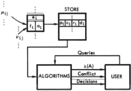
A user asks questions about the current state of the evidence. One set of questions concerns the values of various measures associated with arbitrary A~e . These questions take the form 'what is the value of .\(A)?'. where.\ is one of the functions Bel. m, 0 . P* , or Dou. The other possible queries concern the general state of the inference process. Two examples are 'what is the weight of conflict in the evidence?' and .'is there an A such that m(A)" 1; if so, what is A?'. The o(n) time computations described in this section and in Section 6 answer all these questions.
One more tiny detour is necessary before getting on with the business at hand: it is assumed that subsets of e are represented by a form with the computational nicety of bit-vectors as opposed to, say, unordered lists of elements. The computational aspects of this assumpt ion are: (1) the set membership test takes constant time independent of n and the cardinality of the set; (2) the operators~ · n. U , ·, complementation with respect to e . null , and cardinality compute in o(n) time.
5.1. The Computation of K
From equation (4), K- 1 ·I(nA. ·IIlJn(,~i~nJe; (A;) and the weight of internal conflict among the e; i's log K by definition. Note that there may be conflict between the pairs of J.l; and P; that is not expressed because K is calculated from the point of view of the given e; · Fortunately, the total weight of conflict is simply log[K· DK;): this quantity can be computed in o(n) time if K can be.
In order to calculate K, it is necessary to find the collections of A; that satisfy nA;'~<l2! and e ; (A;)'~'O, i.e., those collections that contribute to the summation. If A; is not {i} , '""'~{i} . or e. then e; = 0 identically from the definition of the simple evidence functions. Therefore. assume throughout that A;E { {i} '""'~{i} e} .
There are exactly two ways to select the A; such that nA; '~<0 .
- If Ai" {i} for some j. and A; = '""'~{i} or A; · e for i'~< j, then nA; " {i}'~<0 . However, if two or more A; are singletons, then the intersection is empty.
- If none of the A; are singletons, then the situation is as follows. Select any s~e and let A; · e when iES and A; · '""'~{i} when i(S. Then nA; · S. Therefore: when no A; is a singleton. nA; '~< 12! unless A;= '""'~{i} for all i.
Let J, K. L be predicates respectively asserting that exactly one A; is a singleton. no A; is a singleton. i.e .. all A;E{..,{i} 9} . and all A, z --,{i} . Then equation (4) can be written as
Now the transformation. below called transformation T,
can be applied to each of the three terms on the right ; after some algebra. it follows that
where P; · e;({i}), C; · e;("""~{i}), and d; " e;(--,{i}) +e;(e) have been substituted. If p "1 for some q, then dQ "c "0 and K- 1 · nli·qJd;· On the ofher hand, if P;'~'1 for all i, then d;~O for all i and equation (5) can be rewritten as
In either case. it is easy to see that the computation is achieved in o(n) time, as is the check for P; · 1.
5 .2. The Computation of m(A)
From equation (4) . the basic probability numbers. m(A) for the orthogonal sum of the simple evidence functions are
for A~ 0 and by definition, m(0) "0. Also. m can be expressed by
It is easy to see that the calculation is achieved in o(n) time since IAI + 1--,AI· n.
Derivation of these formulae is straightforward. If A · nA;. then A~ A; for 1 SiSn and for all j(A, there is an A, such that j~A; · Consider the ·:ase in which A is a nonsingleton nonempty set: If iEA. then A; .. e-the only possibilities are {i) or ""'{i), but neither contains A. II i~A . then both A; = --,{i) and A; = 8 are consistent with A~ A;. However . if A;= e for some i ~A. then nA; ;dAU{i)~A. Therefore. the only choice is A; = '""'~{i) when i~A and A;= e when iEA. When it is noted that e;(e) = r; and e;(""'{i)) = C;, and transformation T is applied. the formula for the nonsingleton case in equation (7) follows .
When A= {q) . there are two possibilities: AQ = e or Aq = {q) . If AQ =e. then the previous argument lor nonsingletons can be applied to just ify the appearance of the term rQn 1 ... qJC;· If Aq = {q) . then for each i~q it is proper to select either A,= 8 or A; = ""'{i) because. leor t1oth choices. A~A;; actuall y. nA, = {q} =A because Aq,. A. Us1ng transformat ion T and not ing that eQ({q}) = Pq and d; = C; + r, gives the term Pqn(,·qJd; in the above and completes the derivation C·l equation (7) .
5.3. The Computations of Bei(A), P*(A), and Oou(A) Since Dou(A) =Bel("·-, A) and P* (A)= 1-Dou(A) . the computation of P* and Dc·u is o(n) if Bel can be computed in o(n) because complementation is an o(n) operation. Let Bel be the orthogonal sum of the n simpie evidence functions. Then Bel(0) = 0 by definition and for A'l<0,
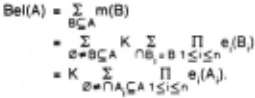
Bel is also expressed by
when d;'l<O for all i. If dq = 0, then Pq = 1. Therefore, m({q}) = Bel({q}) .. 1. In all variations, Bei(A) can be calculated in o(n) time. Since the formula evaluates Bel(0) to 0, only the case of nonempty A needs to be argued.
The tactic is to find the collections of A; satisfying 0;t nA;kA then apply transformation T. Recall that the only collections of A; that satisfy 0:;o nA; are those in which (1) exactly one A; is a singleton or (2) no A; is a singleton and at least one A;= e. To satisfy the current constraint . we must find the subcollections of these two that also satisfy nA;kA.
If exactly one A; is a singleton, say Aq = {q} . then nA; = {q} . In order that nA;kA it is necessary and sufficient that qEA. Thus, the contribution to Bei(A) . when exactly one singleton A; is permitted, is the sum of the contributions for all iEA. A brief computation shows this to be (n[1 $i$n)d;][I[iEA)P/d,].
When no A; is a singleton. it is clear that A, = ...,{i} for ill A; otherwise, iEA, and nA;gA. For iEA. either A,= ...,{i} or A,= 9 is permissible. The value of the contribution to Bel from this case is given by the term [n 1 ,(AJC;)[n 1 ;EAJdJ Since at least one of the A;" e is required, we must deduct for the case in which A,= ...,{i} for all i, and this explains the appearance of the term -n 11 $i$n]C; ·
5 .4. The Computation of Q(A)
The definition of the commonality function shows that 0(0) = 1 identically. For A;t0 .
0 can be expressed also by
In order that a collection, A; , satisfy AknA;. it is necessary and sufficient that AkA; for all i. If i(A, then both A;= ...,{i} and A;" 9 fill this requirement but A;. {i} fails. If iEA, then clearly A;= ...,{i) fails and A; · e works. Further, A; .. {i} works iff A= {i} . It is now a simple matter to apply transformation T and generate the above result. It is evident that O(A) can be calculated in o(n) time.
6. CONFLICT AND DECISIVENESS
In the previous section, a mythical system was introduced that gathered and pooled evidence from a collection of sensors. It was shown how queries such as 'what is the value of >..(A)?' could be answered efficiently. where A is an arbitrary subset of e and >.. is one of Bel. m 0 . P* . or Dou . It is interesting to note that a sensor may change its value over time. The queries report values for the current state of the evidence. Thus. it is easy to imagine an implementation performing a monitoring task. for wh·ch better and more decisive data become available, as time passes. and decisions are reevaluated and updated on the bases of the most current evidence.
In this section, we examine more general queries about the combined evidence. These queries seek the subsets of 9 that optimize one of the measures. The sharpest question seeks the A!;;;9. if any. such that m(A) = 1. If such an A exists. it is said to be the decis ion. Vaguer notions of decision in terms of the other measures are examined too.
The first result is the necessary and sufficient conditions that the evidence be totally contradictory. Since the orthogonal sum of the evidence does not exist in this case. it is necessary to factor this out before the analysis of decisiveness can be realized . All queries discussed in this section can be answered in o(n) time.
6 .1. Totally Contradictory Evidence
Assume there are two or more P, = 1. say p 8 = pb = 1. where a;t b. Then d 1 = c 1 = ri = 0. for both j =a and j =b. The formula for K is
and it is easy to see that K- 1 = 0 under this assumption . Therefore. the evidence is in total conflict by definition .
Let p 8 = 1 and P,'l<1 for i;ta. Then d 8 = c 8 = 0. and d,;t0 for i;ta. Therefore. the above formula reduces to K- 1 = n 1 ,,. 81 d,'l<0 and the evidence is not totally contradictory.
Now assume P;;t 1, hence d;;t0. for all i. Can K- 1 = 0? Since d; = c, + r;. it follows that nd;-nc;;?!:O. If K- 1 = 0. this difference must vanish . This can happen only if r; = 0 for all i. Since p 1 ;t 1. this entails c, = 1 for all i. In this event the P; = 0 and K- 1 = 0.
Summary: The evidence is in total conflict iff either (1) there exists an a'l<b such that both p 8 = pb = 1 or (2) C; = 1 for all i€9 .
6.2. Decisiveness in m
The evidence is decisive when m(A) = 1 for some A!;;;9 and A is called the decision . If the evidence is decisive and A is the decision, then m(B) = 0 when B'l< A because the measure of m is 1. The evidence cannot be decisive if it is totally contradictory because the orthogonal sum does not exist, hence m is not defined. The determination of necessary and sufficient conditions that the evidence is decisive and the search for the decision is argued by cases.
If Pq = 1 for some q€9. then the evidence is totally contradictory if P, = 1 for some i;tq. Therefore, assume that P,;t 1 for i'l<q. From equation (7) it is easy to see m({q}) = Kn 1 ,,.qJd; because rq = 0. Further . it was shown directly above that K- 1 = n 1 ,,.q 1 d, under the sall)e set of assumptions. Thus, m( { q)) = 1.
The other possibility is that P;'l<1 , hence d;'l<O, for all i€9 . Define C = {i(c, = 1 ), and note that if ICI = n. the evidence is totally contradictory. For iEC, P; = r; = 0 and d, = 1. If ICI = n-1 , then there is a w such that {w} = 9-C. Now pw;t1 and c.,;t1 entails rw'l<O; therefore, from equation (7)
If there is a decision in this case. it must be {w} . Direct substitution into equation (5) shows that . in this case. K- 1 = Pw + r w and t~·erefore . m({w)) = 1.
Next . we consider the cases where O~ICI~n - 2 and th~:~refore . I....,CI~2 . Then. from equation (7)
because i~C iff c;-:~:. 1 (and P,-:t:. 1 tor all i€8) has been assumed: hence. r;-:t:.O tor all iE....,C. Therefore. it the evidence is decisive. m(....,C) = 1 is the only nonzero basic probability number. Can there be a Pq-:t:.O? Obviously. q~C. The answer is no since d , -:~:-0 . hence m({q}) = K[pqn[i·q]d; + rqn[i·qJc,]-:t:.O. a contradiction Thus. P; = 0 for all i€8 . From equation (5) it now follows that K- 1 = n[1 :S ·:Sn]d;-n[1:Si:Sn)C;· Therefore. from (9) . n[,~C]r; = n[1 :S·:Sn]d, n[1 :S ·:SnJC; 11 m(....,C) = 1. Since d, = c, = 1 when iEC. this can be rewritten as n[oEC]r, = n [ 1 (qd,-n[oEC)c,. But d, = c, + r, . Therefore. this is possible exactly where c, = 0 when i~C .
Summary : Assuming the evidence IS not in total conflict. it is decisive iff either (1) exactly one P, = 1: the decision is { i} . (2) There exists a w such that cw -:1:.1 and C; = 1 when i-:t:.w: the decision is {w} . Or (3) there exists a W-:t:.0 such that r; = 1 when iEW and C; = 1 when i~W ; the decision is W.
6.3 . Decisiveness in Bel, P*, and Dou
If Bei(A)"' Bei(B) · 1, then Bei(AnB) .. 1 and it is always true that Bel(8)"' 1. The minimal A such that Bei(A) .. 1 is called the core ot Bel. If the evidence is decisive, i.e .. m(A). 1 for some AC8 then clearly A is the core of Bel. Assume the evidence is not de~isive, not totally contradictory, and Bei(A)" 1, then equations (8) and (6) can be smashed together and rearranged to show that
Since the evidence is not decisive, d.-:t:.O. Further. d =c.+ r. so that r; · 0 when i~A: otherwise, the e~pression nd~nc 1 ~akes a I I nonzero contribution to the above. Similarly, P; .. 0 when i ~ A: hence C; · 1 is necessary. Let A= {ilc;-:t:.1}. then substitution shows Bei(A)" 1 and A is clearly minimal .
Summary : The decision is the core when the evidence is decisive, otherwise {ilc;-:1:.1} is the core.
P* and Dou do not give us interesting concepts of decisiveness because Dou(A)" Bei(....,A) = 0 would be the natural criterion. However this test is passed by any set in the complement of the core as well as others. Therefore. in general, no unique decision is found. A similar difficulty occurs in an attempt to form a concept of decisiveness in P* because P* (A)= 1-Dou(A).
6.4. Decisiveness in Q
Since 0(0) = 1 and O(A)~Q(B) when B~A. it is reasonable to ask tor the maximal N such that Q(N) = 1. This set . N. is called the nucleus of Bel. If m(A) = 1, then the decision. A. is clearly the nucleus. If iEN, then iEA for all m(A)-:t:.O. Further . Q({i}) = 1 iff i is an element of the nucleus.
Assume that the simple evidence functions are not totally contrad ictory and there is no decision. Then d;-:t:.O and there is no w such that C;" 1 whenever i-:t:.w. The nectssary and sufficient conditions. then . that Q({z})=1 . and hence zEN are (1) P;=O if ;-:t:.z and (2) Cz · 0. To wit.
Since d;-:1:.0, it follows that Pq = 0 for q-:t:.z, else the first term makes a nonzero contribution . Since d; = c, + r; , the quantity, nd;-nc, . can vanish only if r;=O when i-:t:.z. However. this and p,-:1:-1 . because there is no decision. entails C; = 1 when i-:t:.z. Therefore. either {z} is the decision or the evidence is contradictory. Thus. cz = 0 so that the second term of the last equation vanishes. Since the steps above are reversible, these are sufficient conditions too.
Summary: If A is the decision, then A is the nucleus. If two or more P;-:t:.O. then the nucleus is 0 . If pz-:t:.O. c, = 0, and P; = 0 when i-:t:.z. then {z} is the nucleus. If p 1 = 0 for all i, then {ilc 1 .. 0} is the nucleus. Clearly. this construction can be carried out in o(n) time.
6.5 . Discussion
It has been noted that P; "' 1 or C; = 1 if and only if there is a j such that respectively J.l;i({i}) = 1 or ";i(....,{i}) = 1. i.e .. if and only if the result of some experiment is decisive within its scope. The above analyses show the effects occurring when P; = 1 or C; = 1; subsets of possibilities are irrevocably lost-most or all the nondecisive evidence is completely suppressed-or the evidence becomes totally contradictory.
Any implementation of this theory should keep careful tabs on those conditions leading to conflict and / or decisiveness. In tact , any decisive experiment (a degree of support of 1) should be viewed as based upon evidence so conclusive that no further information can change one's view. A value of 1 in this theory is indeed a strong statement.
7. CONCLUSION
Dempster and Shafer's theory of plausible inference provides a natural and powerful methodology for the representation and combination of evidence. I think it has a proper home in knowledge-based expert systems because of the need tor a technique to represent weights of evidence and the need tor a uniform method with which to reason. This theory provides both. Standard statistical methods do not perform as well in domains where prior probabilities of the necessary exactness are hard to come by. or where ignorance of the domain model itself is the case. One should not minimize these problems even with the proposed methodology. It is hoped that with the ability to directly express i\lnorance and uncertainty. the resulting model will not be so brittle.
However . more work needs to be done with this theory before it is on a solic foundation. Several problems remain as obvious topics for future research . Perhaps the most pressing is that no effective decision making procedure is available. The Bayesian approach masks the problem when priors are selected. Mechanical operations are employed from gathering evidence through the customary expected-value analysis. But our ignorance remains hidden in the priors.
The Dempster-Shaler theory goes about things differently ignorance and uncertainty are directly represented in belief functions and remain through the combination process. When it is time to make a decision, should the estimate provided by Bel or the one provided by P* be used? Perhaps something in between . But what? No one has a good answer to this question.
Thus, the· difference betwee'l the theories is that ~e Bayesian approach suppresses ignorance up front while the other must deal with it after the evidence is in. This suggests one benefit of the Dempster -Shaler approach: surely it must be right to let the evidence narrow down the possibilities. first , then apply some ad hoc method afterward.
Another problem, not peculiar to this theory, is the issue of independence. The mathematical model assumes that belief functions combined by Dempster's rule are based upon inde· pendent evidence, hence the name orthogonal sum. When this is not so, the method loses its feeling of inevitability. Also, the elements of the frame of discernment, 9 , are assumed to be exclusive propositions. However, this is not always an easy constraint to obey. For example, in the MYCIN application. it seems natural to make the frame the set of possible infections but the patient can have multiple infections. Enlarging the frame to handle all subsets of the set of infections increases the difficulty in obtaining rules and in their application; the cardinality of the frame grows from 191 to 21 9 1.
One more problem that deserves attention is computational efficiency. Above it is shown that , with a certain set of assumptions. it is possible to calculate efficiently. However . these assumptions are not valid in all or even most domains. A thorough investigation into more generous assumptions seems indicated so that more systems can employ a principled reasoning mechanism.
The computational theory as presented here has been imple· mented in SIMULA. Listings are available by writting directly to the author.
8.REFERENCES
- J. A. Barnett, Computational Methods for a Mathematical Theory of Evidence: Part II. Forthcoming.
- James Bernoulli. Ars Conjectandi . 1713
- A. P. Dempster, "On direct probabilities," J. Roy. Statist. Soc. Ser. 8 25, 1963, 102·107.
- A. P. Dempster, "New methods for reasoning toward poste· nor distributions based on sample data," Ann. Math. Statis. 37, 1967, 355·37<4.
- A. P. Dempster, "Upper and lower probabilities induced by a multivalued mapping," Ann. Math. Statis. 38, 1967, 325·339.
- A. P. Dempster, "Upper and lower probability inferences based on a sample from a finite univariant population ," Biometrika 54, 1967, 515·528.
- A. P. Dempster, "Upper and lower probabilities generated by a random closed interval," Ann. Math. Statis. 39, (3), 1968. 957·966.
- A. P. Dempster, "A generalization of Bayesian inference." J. Roy. Statis. Soc. Ser. 8 30. 1968, 205·247.
- A. P. Dempster, "Upper and lower probability inferences lor families of hypotheses with monotone density ratios," Ann. Math. Statis. 40, 1969, 953·969.
- R. 0 . Duda, P. E. Hart. and N. J. Nilsson, Subjective Bayesian meth:>ds for rule-based inference systems . Stanford Re· search Institute. Technical Report 124, January 1976.
- 11 . L. Friedman. Extended plausible inference. These proceed· ings.
- T. Garvey. J. Lowrance. M. Fischler, An inference technique for integrating knowledge from disparate sources. These proceedings.
- F. Hayes-Roth and V. R. Lesser. "Focus of Attention in the Hearsay· II Speech-Understanding System." in IJCAI77 . pp. 27·35, Cambridge. MA. 1977.
- H. E. Pople. Jr., "The formation of composite hypotheses in diagr.ostic problem solving: an exercise in synthetic reasc·ning." in Proc. Fifth International Joint Conference on Artificial Intelligence . pp. 1030-1037, Dept. of Computer Science. Carnegie-Mellon Univ .. Pittsburgh. Pa .. 1977.
- G. Sraler, "A theory of statistical evidence." in W. L. Harper and C. A. Hooker (eds.}. Founda rions and Philosophy of Stati~· tical Theories in Physical Sciences. Reidel. 1975.
- G. Sr. a fer, A Mathematical Theory Of Evidence. Princeton University Press, Princeton, New Jersey, 1976.
- E. H. Shortliffe, Artificial Intelligence Series. Volume 2: Computer-Based Medical Consultations: MYCIN , American Elsevier. Inc .· N. Y.,. chapter IV, 1976.
- L.A. Zadeh, "Fuzzy sets," Information and ControlS, 1965. 338<i53.
@inproceedings{ijcai1981p166,
  title     = {Computational Methods for a Mathematical Theory of Evidence},
  author    = {Barnett, Jeffrey A.},
  booktitle = {Proceedings of the Seventh International Joint Conference on
               Artificial Intelligence, {IJCAI-81}},
  publisher = {International Joint Conferences on Artificial Intelligence},
  editor    = {Patrick J. Hayes},
  pages     = {868--874},
  year      = {1981},
  month     = {8},
  note      = {Expert Systems},
  url       = {https://ijcai.org/proceedings/1981/166},
}
TY - CPAPER TI - Computational Methods for a Mathematical Theory of Evidence AU - Barnett, Jeffrey A. T2 - Proceedings of the Seventh International Joint Conference on Artificial Intelligence, IJCAI-81 PB - International Joint Conferences on Artificial Intelligence PY - 1981 SP - 868 EP - 874 UR - https://ijcai.org/proceedings/1981/166 ER -Copied
Machine-readable versions of this paper, for tools and AI agents:





