
Rover Visual Obstacle Avoidance
Proceedings of the Seventh International Joint Conference on Artificial Intelligence. Robotics. Pages 785-789.
© 1981 International Joint Conferences on Artificial Intelligence
Abstract
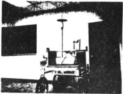
The Stanfdrd AI Lab can is a remotely controlled TV equipped mobile robot A computer program has driven the can through cluttered spaces, gaining its knowledge of the world entirely from images broadcast by the onboard TV system. The can uses several kinds <if stereo to locate objects around it in 30 and to deduce its own motion. It plans an obstacle avoiding path tO a desired destination on the basis of a modei built with this information. The plan changes as the can perceives new obstacles on its journey. The system is reliable for shon runs. but slow. The can moves one meter every ten to fifteen minutes, in lurches. After rolling a meter it stops. takes some pictures and thinks about them for a long time . Then it plans a new path, executes a little of it, and pauses again . It has successfully driven the can through several 20 meter courses (each taking about five hours) complex end\Jgh to necessitate three or four avoiding swerves. Some weaknesses and possible improvements were suggested by these and other, less successful, runs.
Full text extracted automatically from the PDF; figures, tables and equations may differ. The PDF is the version of record.
Rover Visual Obstacle Avoidance
Hans P. Moravec Robotics Institute Ca rnegie·Mellon University
disaster terminates the program. Figure Ia and lb document u1c can's internal world model at two points during a sample run.
CAMERA CALIBRATION
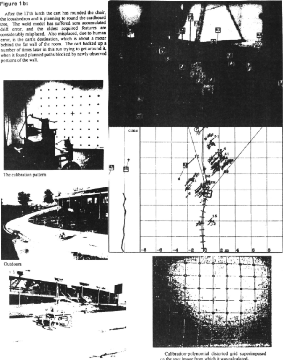
The camera's focal length an geometric distonion arc determined by parking the can a precise distance in front of a wall of many spots and one cross. A program digitizes an image of the spot array, locates the spots and the cross. and constructs a a two dimensional polynomial that relates the position of the spots in the image to their position in an ideal unity focal length camera, and another polynomial that converts points from the ideal camera to points in the image. These polynomials arc used to correct the positions of perceived objects in later scenes.
The algorithm begins by determining the array's approximate spacing and orientation. It trims the picture to make it square, reduces it by averaging to 64 by 64, calculates the Fourier transform of the reduced image and takes its power spectrum, arriving at a 2D transform symmetric about the ·origin, and having strong peaks at frequencies corresponding to the horizontal and venical and half-diagonal spacings. with weaker peaks at the harmonics. It multiplies each point [~Jl in this transform by point[· j.t] and points (Nj+ 1] and [i+ j.j-t]. effectively folding the primary peaks onto one another. The strongest peak in the 90 degree wedge around the y axis gives the spacing and orientation information needed by the next part of the process.
The interest operator described later is applied to roughly locate a spot ncar the center of the image. A special operator examines a window surrounding this position, generates a histogram of intensity values within the window, decides a threshold for separating the black spot from the white background, and calculates the centroid and first and second moment of the spot. This operator is again applied at a displacement from the first centroid indicated by the orientation and spacing of the grid, and so on, the region of found spots growing outward from the seed.
A binary template for the expected appearance of the cross in the middle of the array is constructed from the orientation/spacing data from the Fourier transform. tbe area around each of the found spots is thresholded on the basis of the expected cross area. and the resulting two valued pattern is convolved with the cross template. The closest match in the central ponion of the picture is declared to be the origin.
Two least-squares polynomials (one for X and one for Y) of third (or sometimes founh) degree in two variables, relating the actual positions of the spots to the ideal positions in a unity focal length camera, arc then generated and written into a file. The polynomials arc used in the obstacle a voider to correct for camera roll, tilt, focal length and long term variations in the vidicon geometry.
INTEREST OPERATOR
The cart vision code deals with localized image patches called features. A feature is conceptually a point in the three dimensional world, but it is found by examining localities larger than points in pictures. A feature is good if it can be located unambiguously in different views of a scene. A uniformly colored region or a simple edge is not good because its parts are
Abstract
The Stanfdrd AI Lab can is a remotely controlled TV equipped mobile robot A computer program has driven the can through cluttered spaces, gaining its knowledge of the world entirely from images broadcast by the onboard TV system.
The can uses several kinds <if stereo to locate objects around it in 30 and to deduce its own motion. It plans an obstacle avoiding path tO a desired destination on the basis of a modei built with this information. The plan changes as the can perceives new obstacles on its journey.
The system is reliable for shon runs. but slow. The can moves one meter every ten to fifteen minutes, in lurches. After rolling a meter it stops. takes some pictures and thinks about them for a long time. Then it plans a new path, executes a little of it, and pauses again.
It has successfully driven the can through several 20 meter courses (each taking about five hours) complex end\Jgh to necessitate three or four avoiding swerves. Some weaknesses and possible improvements were suggested by these and other, less successful, runs.
INTRODUCTION
A run of the avoider system begins with a calibration of the cart's camera. The can is parked in a standard position in front of a wall of spots. A calibration program notes the disparity in position of the spots in the image seen by the camera with their position predicted from an idealized model of the situation. It calculates a distonion correction polynomial which relates these positions, and which is used in subsequent ranging calculations.
The can is then manually driven to its obstacle course (littered whith large and small debris) and the obstacle avoiding program is staned. It begins by asking for the can·s destination, relative t9 its current position and heading. After being told, say. SO meters forward and 20 to the right, it begins its maneuvers. It activates a mechanism w_hich _moves_ the TV camera. and digitizes nine pictures as the camera shdcs m prec1se steps from one side to the other along a SO em track.
A subroutine called the interest operator is applied to the one of these pictures. It picks out 30 or so particularly distinctive regions (features) in this picture. Another routine called ihe co"ela1or looks for these same regions in the other frames. A program called the camera solver determines the three dimensional position of the features with respect to the can from their apparent movement image to image.
The navigator plans a path to the destination which avoids all the perceived features by a large safety margin. The program then sends steering and drive commands to the can to move it about a meter along the planned path. The can's response to such commands is not very precise. The camera is then operated as before, and nine new images are acquired. The control program uses a version of the corrclator to find as many of the features from the previous location as. possible in the new pictures. and applies the camera solver. The program then d~duc~ the can's actual motion during the step from the apparent three dJmens1onal shift of these features. Some of the features arc pruned during this process. and the interest operator is invoked to add new ones.
This repeat~ until the can arrives at its destination or until some indistinguishable. Regions such as comers. with high contrast in orthogonal directions are best New features in images are picked by a subroutine called the interest opt>rator. It tries to select a relatively unifonn scattering of good features, to maximize the probability that a few features will be picked on every visible object by returning regions that arc local maxima of a directiona1 variance measure. Featureless areas and simple edges, which have no variance in the directior of the edge, are thus avoided.
Directional variance is measured over small square windows. Sums of squares of differences of pixels adjacent in each of four directions (horizontal. vertical and two diagonals) over each window are calculated, and the window's interest measure is the minimum of these four sums. Features are chosen where the· interest measure has local maxima. The chosen features are stored in an array. sorted in order of decreasing interest measure.
Once a feature is chosen, its appearance is recorded as series of excerpts from the reduced image sequence. A w,indow (6 by 6 in the current implementation) is excised around the feature's location from eacli of the variously reduced pictures. Only a tiny fraction of the area of the original (unreduced) image is extracted. rour times as much of the x2 reclnced image is stored, sixteen times as much of the x4 reduction. and so on until at some level we have the whole image. The final result is a series of 6 by 6 pictures. beginning with a very blurry rendition of the whole picture, gradually zooming in linear expansions of two to a sharp closeup of the feature.
Weaknesses
The measure is able to unambiguously reject edges only if they are oriented along the four directions of summation. Edges with intenncdiate direction give non-zero values for all four sums. and are sometimes incorrectly chosen as interesting. The operator especially favors intersecting edges. These arc sometimes comers or cracks in objects, and are very good. Sometimes they arc caused by a distant object peering over the edge of a nearby one and then they are very bad. Such spurious .ntcrsections do not have a definite distance, and must be rejected during camera solving.
CORRELATION
Deducing the 30 location of features from their projections in 20 images requires that we know their ~ition in two or more such images. The co"tlatofis a subroutine that, given a feature description produced by the interest operator from one image, finds the best match in a different. but similar, image. Its search area can be the entire new picture, or a rectangular sub-window.
The search uses a coarse to fine strategy that begins in reduced versions of the pictures. Typically the first step takes place at the x16 (linear) reduction level. The 6 by 6 window at that level in the feature description, that covers about one seventh of the total area of the original picture, is convolved with the search area in the correspondingly reduced version of the second picture. 'llle 6 by 6 description patch is moved pixel by pixel over the approximately 15 by 16 destination picture. and a correlation coefficient is calculated for each trial position. The position with the best match is recorded. The 6x6 area it occupies in the second picture is mapped to the x8 reduction level, where the corresponding region is 12 p1xels by 12. llte 6 by 6 window in the x8 reduced level of the feature description is then convolved with this 12 by 12 area, and the position of best match is recorded and used as a search area for the x4 level. The process continues, matching smaller and smaller, but more and more detailed windows until a 6 by 6 area is selected in the unreduced picture. 'lbc window sizes and other parameters are sometimes different from the ones used in this example.
STEREO
Slider Stereo
At each pause on its computer controlled itinerary the cart slides its camera from left to right on the 52 em track, taking 9 pictures at precise 6.5 em intervals. Points are chosen in the fifth (middle) of these 9 images, either by the correlator to match features from previous positions,.or by the interest operator. 'lbe camera slides parallel to the horizontal axis of the (distortion corrected) camera co-ordinate system. so the parallax· induced displacement of features in the 9 pictures is purely horizontal.
The correlator looks for the points chosen in the central image in each of the eight other p1ctures. 'The search is restricted to a narrow horizontal band. This has little effect on the computation time, but it reduces the probability of incorrect matches. In the case of correct matches, the distance to the feature is inversely proportional to its displacement from one image to another. The uncertainty in such a measurement is the difference in distance a shift one pixel in the image would n:take. The uncertainty varies inversely with the physical separation of the camera positions where the pictures were taken (the stereo baseline). Long baselines give more accurate distance measurements.
After the correlation step the program knows a feature's position in nine images It considers each. of the 36 ( = 9 choose 2) possible image pairings as 2 stereo baseline, and records the estimated (inverse) distance of the feature in a histogram. F.ach measurement adds a little nonnal curve to the histogram. with mean at the estimated distance, and standard deviation inversely proportional to the baseline, reflecting the uncertainty. The area under each curve is made proportional to the product of the correlation coefficients of the matches in the two images (in central unage this coefficient is taken as unity), reflecting the confidence that the correlations were correct. The distance to the feature is indicated by the largest peak in the resulting histogram, ;f this peak is ahove a certain threshold. If below, the feature is forgotten about.
The correlator sometimes matches features incorrectly. llte distancco measurements from incorrect matches in different pictures are not consistent When the nonnal curves from 36 pictures pairs arc added up, the correct matches agree with each other, and build up a large peak in the histogram, while incorrect matches spread themselves more thinly. Two or three correct correlations out of the eight will usually build a peak suffiCient to offset a larger number of errors. In this way eight applications of a mildly reliable operator interact to make a very reliable distance measurement
Motion Stereo
After having detennined the 30 location of objects at one position, the computer drives the cart about a meter forward. At the new position it slides the camera and takes nine pictures. 'lllc correlator is applied in an attempt to find all the features successfully located at the previous position. Feature descriptions extracted from the central image at the last position arc searched for in the central image at the new stopping place.
Slider stereo then dctennines the distance or the features so found from the cart's new position. The program now knows the 3D position· of the features relative to its camera at the old and the new locations. Its own movement is deduced from 3D co-ordinate transfonn that relates the two.
The program first eliminates mis-matches in the correlations between the central images at two positions. Although it oocsn't yet have the co ordinate uansfonn between the old and new camera systems. the program knows the distance between pairs of feature positions should be the same in both. It makes a matrix in which element [~Jl is the aosolute value or the diffcrcnrc in distances between points i and j in the first and second co-ordinate systems divided by the eKpected error (based on the one pixel uncertainty of the ranging). Each row of this matrix is summed, giving an indication of how much each point disagrees with the other points. 'llle idea is that while points in error disagree with virtually all points, correct positions agree with all the other correct ones, and disagree only with the bad ones. The worst point is deleted, and its effect is removed from the remaining points in the row sums. This pruning is repeated until the worst error is within the error expected from the ranging uncertainty.
After the pruning, the program has a number of points, typically 10 to 20, whose position error is small and pretty well known. The program trusts these, and records them in its world model, unless it had already done so at a previous position. The pruned points arc forgotten forevermore.
The 3d rotation and translation that relates the old and new cart position is t!Jcn calculated by a Newton's method iteration that minimizes the sum of the squares of the distances-between the transformed first co· ordinates and the raw co-ordinates of the corresponding points at the second position. w1th each term divided by the square of the expected unccllainty in the 3D position of the point~ involved.
PATH PLANNING
The cart vision system "models" objects as simple clouds of features. If enough features arc found on each nearby object. this model is adequate for planning a non-colliding path to a destination. The features in the cart's 3D world model can be thought of as fu7.ly ellipsoids. whose dimensions r<'flect the program's uncertainty of their position. Repeated applications of the i11tcrest operator as the cart moves cause virtually all visible objects to be become modelled as clusters of overlapping ellipsoids.
To simplify the problem. the ellipsoids arc approximated by spheres. Those spheres sufficiently above the Ooor and below the cart's maximum hciRht arc projected on the noor as circles. The can itself is modelled as a 3 meter circle. The path finding problem then becomes one of maneuvering the cart's 3 meter circle between the (usually smaller) circles of the potential obstacles to a desired location. It is convenient (and equivalent) to conceptually shrink the cart to a point. and add its radius to each and· every obstacle. An optimum path in this epvironmcnt will consist of either a straight run between start and finish. or a series of tangential segments between the circles and· contacting arcs (imagine loosely laying a string from start to finish between the circles, then pulling it tight).
The program converts the problem to a shortest path in graph search. There arc four possible paths between each pair of obstacles because each tangent can approach clockwise or counterclockwise. Each tangent point becomes a vertex in the graph, and the distance matrix contains sums of tangential and arc paths. with infinities for blocked or impossible routes. The cart program was occasionally run using this exact procedure, but more. often with a faster approximation that made each obstacle into two vertices (one for each direction of circumnavigation).
A few other considerations were essential in the path planning. The charted routes consist of straight lines connected by tangent arcs, and are thus plausible paths for the cart. which steers like an automobile. This plausibility is not necessarily true of the start of the planned route, which, as presented thus far, does not take the initial heading of the cart into account. The plan could. for instance. include an initial segment going off 90 degrees from the direction in which the cart points. and thus be impossible to execute. This is handled by including a pair of "phantom" obstacles along with the real perceived ones. The phantom obstacles have a radius equal to the cart's minimum steering radius. and arc placed, in the planning process. on either side of the cart at such a distance that after their radius is augmented by · the cart's radius (as happens for all the obstacles). they just touch the cart's centroid. and each other, with their common tangents being parallel to the direction of the cart's heading. They effectively block the area made inaccessible to the cart by its maneuverability limitations.
Path Execution
After the path to the destination has been chosen. a portion of it must be implemented as steering and motor commands and transmitted to the cart. The control system is primitive. The drive motor and steering motors may be turned on and off at any time, but there exists no means to accurately determine just how fast or how far they have gone. The current program makes the best of this bad situation by incorporating a model of the cart that mimics. as accurately as possible, the cart's actual behavior. Under good conditions. as accurately as possible means about 20%; the cart is not very repeatable. and is affected by ground· slope and texture. battery voltage, and other less obvious externals.
The path executing routine begins by excising the first .75 meters of the planned path. ·n1is distance was chosen as a compromise between average cart velocity. and continuity between picture sets. If the cart moves too far between picture digitizing sessions. the pitture will change too much for reliable correlations. This is especially true if the cart turns (steers) as it moves. The image seen by the camera then pans across the field of view. The cart has a wide angle lens that covers 60 degrees horizontally. 'llle .75 meters. combined with the turning radius limit (5 meters) of the cart results in a maximum shift in the field of view of 15 degrees. one quarter of the entire image.
The program examines the cart's position and orientation at the end of the desired .75 meter lurch, relative to the starting position and orientation. The displacement is charactcri1.ed by three parameters; displacement forward, displacement to the right and change in heading. In closed form the program computes a path that will accomplish this movement in two arcs of equal radius, but different lengths. The resulting trajectory has a general "S" shape. Rough motors timings arc derived from these paratmetcrs. The program then uses a simulation that takes into account steering and drive motor response to iteratively refine the solution.
CONt;LI.ISION
Many years ago I chose the line of research described herein intending to produce a combination of hardware and software by which the cart could visually navigate reliably in most environments. For a number of reasons. the existing system is only a first approximation to that youthful ideal.
One of the most serious limitations is the excruciating slowness of the program. In spite of my best effort~. and many compromises, in the interest of speed. it takes 10 to 15 minutes of real time to acquire and consider the images at each lurch, on a lightly loaded KL-10. This translates to an effective cart velocity of 3 to 5 meters an hour. Interesting obstacle courses (2 or three major obstacles, spaced far enough apart to permit passage within the limits of the cart'ssilC and maneuverability) are. at least 15 meters long, so interesting cart runs take from 3 to 5 hours, with little competition from other users, impossibly· long under other conditions.
During the last lew weeks of the AI lab's residence in the D.C. Power building, when the full fledged obstacle runs described here were executed, such conditions of light load were available on only some nights, between 2 and 6 AM and on some weekend mornings. ·~e cart's video system battery lifetime on a full charge is at most 5 hours, so the limit~ on field tests, and consequently on the debug/improve loop, were strictly circumscribed.
Although major portions of the program had existed Jnd been debugged for several years, the complete obstacle avoiding system (including fully working hardware, as well as programs) was not ready until two weeks before the lab's scheduled move. The first week was spent quashing unexpected trivial bugs, causing very silly cart behavior under various conditions, in the newest parts of the code, and rccalibrating camera and motor response models.
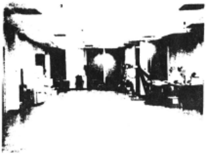
The final week was devoted to serious observation (and filming) of obstacle runs. Three full (about 20 meter) runs were completed, two indoors and one outdoors. Two indoor false starts, ahortcd by failure of the program to perceive an obstacle, were also recorded. ·~e two long indoor runs were nearly perfect
In the first, the cart successfully slalomed its way around a chair, a large cardboard icosahedron, and a cardboard tree then. at a distance of about 16 meters. encountered a cluttered wall and backed up several times trying to find a way around it.
The second indoor run involved a more complicated set of obstacles, arranged primarily into two overlapping rows blocking the goal. llle cart backed up twice to negotiate the tight turn required to go around the first row. then executed several steer forward I back up moves. lining itself up to go through a gap barely wide enough in the second row. This run had to be terminated, sadly, before the cart had gone through the gap because of declining battery charge and increasing system load.
The outdoor run was less successful. It began well: in the first few moves the program correctly perceived a chair directly in front of the camera. and a number of more distant cardboard obstacles and sundry debris. Unfortunately, the program's idea of the cart's own position became increasingly wrong. At almost every lurch, the position solver deduced a cart motion considerably smaller than the actual move. By the time the cart had rounded the foreground chair, its position model was -so far off that the distant obstacles were replicated in different positions in the cart's confused world model, because they had been seen early in the run and again later. to the point where the program thought an actually existing distant clear path was blocked. I restarted the program to clear out the world model when the planned path became too silly. At that time the cart was four meters in front of a cardboard icosahedron, and its planned path lead straight through it. The newly re-incarnated program failed to notice the obstacle, and the cart collided with it. I manually moved the icosahedron out of the way, and allowed the run to continue. It did so uneventfully, though there were continued occasional slight errors in the self position deductions. The cart encountered a large cardboard tree towards the end of this journey and detected a portion of it only just in time to squeak by without colliding.
The two short abortive indoor runs involved setups nearly identical to the two-row successful long run described one paragraph ago. The first row, about three meters in front of the cart's starting position contained a chair, a real tree (a small cypress in a planting pot}, and a polygonal cardboard tree. The cart saw the chair instantly and the real tree after the second move. but fa1led to sec the cardboard tree ever. Its planned path around the two obstacles it did sec put it on a collision course with the unseen one. Placing a chair just ahead of the cardboard tree fixed the problem. and resulted in a successful run. Never. in all my expciicnce, has the code described in this thesis failed to notice a chair in front of the cart.
Flaws Found
These runs suggest that the system suffers from two serious weaknesses. It docs not sec simple polygonal (bland and featureless) objects reliably, and its visual navigation is fragile under certain conditions. Examination of the program's internal workings suggests some causes and possible solutions.
Bland Interiors
The program sometimes fails to sec o!Jstaclcs Jacking sufficient high contrast detail within their outlines. In this regard, the polygonal Lree and rock obstacles I whimsically constructed to match diagrams from a 3D drawing program. were a terrible mistake. In none of the test runs did the programs ever fail tu ·cc a wair placed in front of the cart, but half the time they did fail to sec a pyramidal tree or an icosahedral rock made of clcau white cardboard. These contrived obstacles were picked up reliably at a distance of 10 to 15 meters. silhoueucd against a relatively unmovin& (over slider travel and cart lurches} background, but were only rarely and sparsely seen at , closer range, when their outlines were confused by a rapidly shifting background. and their bland intcrio{s provided no purchase for the interest operator or correlator. Even when the artificial obstacles were correctly perceived, it was by virtue of only two to four features. In contrast, the program usually tracked five to ten features on nearby chairs.
In th~ brightly sunlit outdoor run the artificial obstacles had another problem. Their white coloration turned out to be much brighter than any "naturally" occurring extended object. These super bright, glaring, surfaces severely taxed the very limited dynamic range of the cart's vidicon/digitizer combination. When the icosahedron occupied 10% of the camcm's field of view, the automatic target voltage circuit in the electronics turned down the gain LOa point where the background behind the icosahedron appeared nearly solid black.
Confused Maps
The second major problem exposed by the runs is glitches in the cart's self-position model. This model is updated after a lurch by finding the 3D
translation and rotation that best relates the 3d position of the set of tracked features before and after the lurch. In spite of the extensive pruning that precedes this step, (and partly b~cause of it, as is discussed later) small errors in the measured feature positions sometim-es cause the solver to converge to the wrong transform. giving a position error beyond the expected uncertainty. Features placed into the world model before and after such a glitch will not be in the correct relative positions. Often an object seen before is seen again after, now displaced, with the combination of old and new positions combining to block a path that is in actuality open.
This problem showed up mainly in the outdoor run. I've also observed it indoors in past. in simple mapping runs, before the entire obstacle a voider was assembled. There appear to be two major causes for it, and a wide range of supporting factors. ·
Poor seeing, resulting in too few correct correlations between the pictures before and after a lurch. is one culprit. The highly redundant nine eyed stereo ranging is very reliable. and causes few problems, but the non-redundant correlation necessary to relate the position of features before and after a lurch. is error prone. Sometimes the mutual-distance invariance pruning that follows is overly agrcssivc, and. leaves too few points for a stable least-squares co-ordinate fit.
The outdoor runs encountered another problem. "lbe program ran so slowly that shadows moved significantly (up to a half meter) between lurches. 'lbcir high contrast boundaries were favorite points for tracking, enhancing the program's confusion.
Simple Fixes
'!bough elaborate (and thus far untried in our context} methods such as edge matching may greatly improve the quality of automatic vision in future. subsequent experiments with the program revealed some modest incremental improvements that would have solved most of the problems in the test runs.
The issue of unseen cardboard obstacles turns out to be partly one of over-conservatism on the program's part. In all cases where the can collided with an obstacle it had correctly ranged a few features on the obstacle in the prior nine-eyed scan. 'lbe problem was that the much more fragile correlation between vehicle forward moves failed, and the points were rejected in the mutual distance Lest. Overall the nine-eyed stereo produced very few errors. If the path planning stage had used the pre-pruning features (still without incorporating them permanently into the world model) the runs would have proceeded much more smoothly. All of the most vexing false negatives, in which the program failed to spot a real obstacle, would have been eliminated. There would have been a very few false positives, in which non-existent ghost obstacles would have been perceived. One or two of these might have caused an unnecessary swerve or backup. But such ghosts would not pass the pruning stage, and the run would have recovered after the initial. non-catastrophic, glitch.
The self-position confusion problem is related. and in retrospect may be considered a trivial bug. When the path planner computes a route for the cart, another subroutine lakes a portion of this plan and implements it as a sequence of commamls to be transmiued to the cart's steering and drive motors. During this process it runs a simulation that models the cart acceleration. rate of turning and so on, and which provides a prediction of the cart's position after the move. With the current hardware the accuracy of this prediction is not great. but it nevertheless provides much a priori information about the cart's new position. lbis information is used. appropriately weighted, in the least-squares co-ordinate system solver that deduces the cart's movement from the apparent motion in 3D of tracked features. It is not used. however. in the mutual distance pruning step that prcceeds this solving. When the majority of features have been correctly tracked. failure to usc this infom1a1ion docs not hurt the pruning. But when the seeing is poor, it can niakc the difference between choosing a spuriously agreeing set .of mis-trackcd features and the small correctly matched set
Incorporating the prediction into the pruning, by means of a heavily weighted point that the program treats like another tracked feature, removes almost all the positioning glitches when the program is fed the pictures from the outdoor run.
Figure 1a:
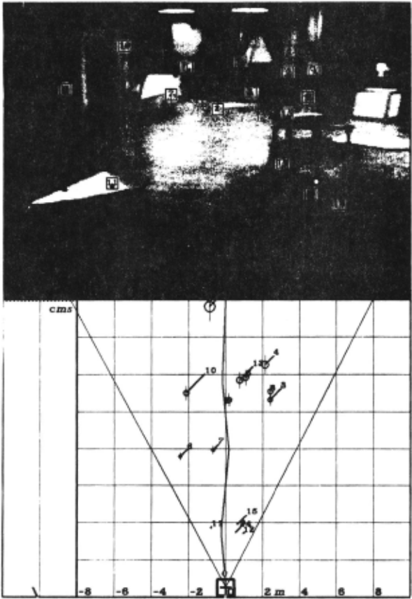
This and the following diagram arc plan views of the cart's world model at obstacle run stopping positions.
In this first view. one step into a run. the cart has (by the program's reckoning) travelled a little under a meter. The program has noted a number of objects: a chair in the foreground. pieces of cardboard on ihc floor, an icosahedron, a refrigerator, a cardboard tree, and some other things. It has deduced that the chair, the icosahedron and the tree arc real obsmcles, and has planned a path which slaloms around them (the cardboard in the foreground has been ignored because it lies on the floor).
The grid cells are two meter squares, conc~tually on the floor. lhe cart's own position is indicated by the small heavy square. and by the graph, indicating height, calibrated in centimeters, to the left of grid. Since the cart never actually leaves or penetrates the floor, this grapn provides an indication of the overall accuracy. The irregular, tick marked, line behind the cart's position is the past itinerary of the cart as deduced by the program. Each tick marie represents a stopping place. The picture at top of the diagrams is the view seen by the TV camera. The two rays projecting forward from the cart position show the horizonml boundaries of the camera's field of view (as deduced by the camera calibration program). 'Inc numbered circles in the plan view arc. features located and tracked by the program. The centers of the circles arc the vertical projections of the feature positions onto the ground. lhc sile of each circle is the uncertainty (caused by finite camera resolution) in the feature's position. 'lhe length of the 45 degree line projecting to the upper right, and terminated by an identifying number, is the height of the feature above the ground, to the same scale as the floor grid. lhc features arc also marked in the camera view. in the guise of numbered bo~cs. The thin line projecting from each bo~ to a lower blob is a stalk which just reaches the ground, in the spirit of the 45 degree lines in the plan view. The irregular line radiating forwards from the cart is the planned future path. This changes from stop to stop, as the cart fails to obey instructions properly, and as new obstacles arc detected. The small ellipse a short distance ahead of the cart along the planned path is the planned position of the nc~t stop ..
@inproceedings{ijcai1981p151,
  title     = {Rover Visual Obstacle Avoidance},
  author    = {Moravec, Hans P.},
  booktitle = {Proceedings of the Seventh International Joint Conference on
               Artificial Intelligence, {IJCAI-81}},
  publisher = {International Joint Conferences on Artificial Intelligence},
  editor    = {Patrick J. Hayes},
  pages     = {785--789},
  year      = {1981},
  month     = {8},
  note      = {Robotics},
  url       = {https://ijcai.org/proceedings/1981/151},
}
TY - CPAPER TI - Rover Visual Obstacle Avoidance AU - Moravec, Hans P. T2 - Proceedings of the Seventh International Joint Conference on Artificial Intelligence, IJCAI-81 PB - International Joint Conferences on Artificial Intelligence PY - 1981 SP - 785 EP - 789 UR - https://ijcai.org/proceedings/1981/151 ER -Copied
Machine-readable versions of this paper, for tools and AI agents:





