A Feature-Based Scene Matcher

ABSTRACT

A method is presented for matching two scene descriptions, each of which consists of a set of measured feature vectors with estimated uncertain­ ties. The two scenes differ by a transformation that depends on a few unknown parameters. The method performs a search by sequentially matching features of one scene to those of the other scene, solving for the transformation parameters by means of a generalized least-squares adjustment, comput­ ing the probabilities of these matches by means of Bayes' theorem, and using these probabilities to prune the search. An example is given using scene descriptions of the Martian surface in which the features are rocks approximated by ellipsoids.

INTRODUCTION

A common problem in vision is that of match­ ing. This may involve matching one two-dimen­ sional image to another, matching a three-dimen­ sional object to its two-dimensional projection, or matching two three-dimensional descriptions of the same scene. For want of a better term, the entities to be matched will be called "scenes". In general, the two scenes may be related in var­ ious complicated ways . For example, there may be "rubber sheet" distortion [1), there may be inde­ pendent changes in different parts of the scene as in the stereo matching problem [2], or there may be arbitrary changes in the different portions of a complicated object as in matching to a generic model [3]. However, in this paper the problem is restricted to the case in which the relation­ ship between the scenes to be matched can be ex­ pressed by a few parameters, each of which has a global effect . Restricting the problem in this way allows the use of robust, efficient techniques that would not be applicable in the more general case.

It is further assumed here that the matching will be done by using local features that have been detected in each scene, that the a priori

*The work described in this paper was started at Stanford University and was completed at the Jet Propulsion Laboratory , Calif omia Institute of Technology, under contract with the National Aeronautics and Space Administration.

A FEATURE-BASED SCENE MATCHER

"'

Donald B. Gennery

Robotics and Teleoperator Group Jet Propulsion Laboratory Pasadena, California 91103

correspondence between features in the two scenes is unknown, that each feature is described by a vec­ tor of measured feature parameter values, and thst for each feature the probability distribution of its measured feature vector values is known. Al­ though in principle any probability density func­ tion of errors in the feature vector could be used, the following treatment is restricted to the spe­ cial case in which the error distribution is de­ termined by its covariance matrix. The possibil­ ity exists that a feature detected in one scene ~1ill not be detected in the other, and this possi­ bility is covered by estimates of probability of detection based on experience.

For example, consider the matching of two aerial photographs which differ by an unknown translation, rotation, and scale factor. In this case four parameters determine the transformation. The features might be local landmarks whose two­ dimensional position and orientation have been measured, in which case each feature vector would have three components. Another example might be recognizing in a two-dimensional image the projec­ tion of a known three-dimensional object. Six parameters determine the position and orientation of the object. The features might be markings, corners, or edges that are known in the object model but must be found in the image.

For a third example, consider an object find­ er [2, 4] which produces a description of a three­ dimensional scene in terms of objects represented by ellipsoids. Thus each feature vector consists of the nine parameters that define the ellipsoid. Suppose that the same area has been viewed from two different locations by a roving vehicle. There will be a partially unknown translation and per­ haps rotation (requiring six parameters in genera~ between tne coordinate systems of the resulting two scene descriptions, caused by errors in the navigation system of the vehicle. It is desired to match these two descriptions in order to cor­ rect the navigation data. (This special case is discussed further elsewhere [2], and an example of its use is presented later in this paper.)

By using the probability distributions of the feature vectors, it is possible to find the opti­ mum matching of the scene in an efficient way that does not consider all possible matches of indivi­ dual features and yet does not overlook matches that nave an appreciable chance of turning out to be correct, In this regard the method to be pre­ sented can be considered to be an improvement over the method of Price [5] and the suggestion of Milgram and Bjorklund [6]. It also has some over­ lap with the method of Fischler and Elschlager [ 1] , lying somewhere between their dynamic programming method and their linear embedding algorithm. (In their terminology, a "spring" would connect each feature to some constant point in the scene for the problem stated above. This is not the kind of situation for which their method was designed to work well.)

It is assumed below that the matching of fea­ tures is one-to-one (with perhaps some features left unmatched) and that all features are of the same type (so that a feature in one scene can be matched to any feature in the other scene). How­ ever, the mathematics can be generalized to the case where several features in one scene can be matched to the same feature in the other scene and to the case where there are different types of features that cannot be matched to each other (with perhaps a different size of feature vector for each type).

NOTATION

Matrix notation will be used. (Hohn [7] pro­ vides a good text on matrix algebra.) For any ma­ trix A, its transpose is denoted by AT, its in­ verse by A-1, and its determinant by det(A). Vec­ tors (of any size) are represented by column ma­ trices. The covariance matrix of any vector X is defined in the usual way to be

• t ((X-eX) (X- eX) T], where e is the mathematical expectation operator. A partial derivative matrix of a vector Y with respect to a vector X is defined so that the rows correspond to elements of Y and the columns correspond to elements of X.

The two given scene descriptions are called Scene A (composed of features Al, A2, etc.) and Scene B (composed of features Bl, B2, etc.). For each feature of each scene the following are give~ with subscripts to denote particular features:

• X · measured feature vector.
• · covariance matrix of X.
• b · probability that the feature will be present in a matching scene.
• r · a priori probabllity density of feature vector for typical scenes, evaluated at X but not otherwise using measured data.

(It is necessary that the dimensionality of Scene B be at least as great as that of Scene A, so that any feature in Scene B can be uniquely projected into Scene A if the transformation is known.)

The following global quantities are given:

• p 0 · a priori probability that the two scenes match (that is, represent the same phy­ sical scene).
• G 0 · a priori estimate of vector of parame­ ters used in the transformation from Scene B to Scene A.
• ro - covariance matrix of G 0 ·
• It is desired to compute the following:
• p · probability that the scenes actually match.
• G · vector of transformation parameters (if the scenes match),
• r · covariance matrix of G.

The following definitions will be needed:

• F(G,XBj) · feature Bj projected from Scene B into Scene A, wnere the multidimens·ional function F is derivable from the known transformation between scenes and the definition of the feature vector.
• Pj · partial derivative matrix of F(G,XBj) with resoect to G.
• R · partial derivative matrix of F(�,~j) j with respect to ~j'
• (Ai,Bj) · pair denoting match of feature Ai to feature Bj.
• M · set of (Ai,Bj) pa~rs for a possible mat­ ching of the two scenes (empty if no pairs are matched) .

MA · set of Ai' s contained in the members of M.

~ a set of Bj 's contained in the members of M.

• m · number of (Ai,Bj)pairs in M.
• a · number of parameters in a Scene-A fea­ ture vector (size of XAi).
• g · number of transformation parameters (size of G).

The symbol E denotes set membership.

Some important intermediate quantities are defined as follows:

• nM = a priori probability that M would occur, given that the scenes match but ignor­ ing the measured feature vectors.
• PM · joint prooability densi.ty of the feature vectors evaluated at the observed values, given that M is the correct matching .
• p 0 · a priori joint probability density of the the feature vectors.
• a posteriori probability of the scenes matching and M being the correct s.et of matches, given the observed feature vec ­ tors.

Other intermediate q\lS.n.ti_tie.£ are defined as needed.

OPTIMUM MATCH

The method to be used involves producing ten­ tative matches of the features in one scene to those in the other and for each match M computing the a priori probability nM, computing the trans­ formation vector GM, and comparing the residuals of the fit to the given feature vector distribu­ tions to evaluate the probability density PM· Then Bayes' theorem is used to compute the a posteriori probability PM· The M for which PM is near unity, if any, can be assumed to be the correct match, and the corresponding GM can be used for G.

Thus the a posteriori probability of M is co~ puted by means of Bayes' theorem as follows:

since Po'~~M is the a priori probability of the scene matching according to M, l-p 0 is the proba­ bility of the scenes not matching, and PM and p 0 respectively are the probability densities that the observed results (feature vectors) would follow from .these events. (It would appear that all com­ binations of feature matches would have to be used in this computation, but a way of avoiding this will be described in the next section.) It remains to describe the computation of 'liM' PM and p 0 ·

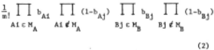
The 'liM quantities needed in {1) can be found by the following reasoning. The probability that feature Ai will be matched to some feature in Scene B is bAi , the probability that it will be unmatched is 1-bAi· and similarly for bBj and 1-bBj for feature number j in Scene B. Thus the probability of a particular subset of m features from Scene A and m features from Scene B being matched, and no others, is the product of these terms over all features, chosen according to whe­ ther each feature is matched or not. However, there are m! ways of matching a set of m features to another set of m features (since the matching is assumed to be one-to-.one). Therefore, this product is divided by m! to obtain the a priori probability of an individual matching combination. Thus

'liM ·

The solution for the G parameters for a par­ ticular matching is computed as follows. An ap­ proximation to G, denoted by G', is used to com­ pute the partial derivative matrices P and R of the transformation F(G' ,XB) as defined in the Notation section. (Note that P and R are implicit functions of G' and XB, in general.) Then for this approximation a discrepancy vector U and its co­ variance matrix T for each matching of feature Ai with feature Bj is computed as follows:

The solution for the parameters can be obtained by a generalized least-squares (minimum-variance) adjustment according to the general method des­ cribed in [8) or in Appendix A of [2], which pro­ duces the maximum-likelihood solution if the errors have the normal (Gaussian)distribution.

(This is only approximately correct here because of the fact that the parameters being adjusted affect the weights through Rj in (4) .) Thus,

If F is nonlinear, the above process may need to be iterated. (G' would be Go on the first itera~ tion but later would be ~ from the previous iter~ tion.)

The above solution can be used to obtain PM for use in (1), provided that the distribution of the measurement errors is known. First,the resi­ duals are

If the errors are normally distributed, the multi­ variate normal distribution produces the following probability density Pij:

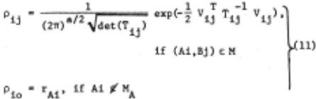
where Pio is for the case in which feature Ai is un­ matched. It includes the a priori distribution of Scene A features only, to be consistent with the discrepancies being computed in Scene A coordi­ nates according to {3). {Strictly speaking, Pij for matched features should include the effects of the a priori distribution also. However, since the a priori distribution is usually much wider than that given by T, this usually would have little effect.) Then,the probability density for the com­ plete match is the product of all of the Pij val­ ues in this combination times the probability den­ sity function of the a priori parameter values, as follows:

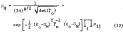
where the product is over all objects in Scene A.

An alternative way of computing PM is possible that may be more efficient than the above. Subst~ tuting (ll) into (12) and combining the exponen­ tial functions produces an equation with the sum"' T -1 mation ~ Vij Tij Vij in the exponent, where an extra term in the summation represents the a pri­ ori parameter values by letting V0 · G0 - GM and T0 - f 0 . This summation is the quadratic form which was minimized in the adjustment, and it can be shown [9] that this is equal to

"' T -1 T ~Uij Tij Uij - DMCM, where as before the a priori parameter values are included in the sum­ mation by letting U0 · G 0 - G'. Therefore, (12) is equivalent to the following when the errors have the normal distribution:

these to unmatched features in Scene B. The a posteriori probability of each of these partial M combinations is computed, and those with negligi­ bly small probability are not pursued further. In this way a search tree is built up, branching out as different features in Scene B (including no feature) are matched to the current feature in Scene A at each level. The features in Scene A can be ordered according to a criterion based on their feature vectors so that those most likely to be unambiguously matched are matched first. Some kind of best-first search could be used, but in order to take advantage of Bayes' theorem in com­ puting the probabilities for pruning the search, a breadth-first search is ·used instead.

Because, when a tentative match is made, it is not known which features in Scene B will remain unmatched, there is no obvious way to use all of the information in (2). Instead, WM is computed by the following recursive method for the purposes of the search, where i now denotes a sequential numbering of Scene A features in the order in which they are selected for matching:

The 'llf. values from (16) are used for 11M in ( 1) for this particular node at the ith level of the search tree,with the other quantities in (1) being computed as described in the previous section,for this partial match. The resulting PM probabili­ ties are used to prune the search.

The criterion used for pruning ideally should not use a constant probability threshold, but should take into account the fact that, if a large number of nodes have small probability each but sum to a large probability, there is a good chance that one of them will turn out to be part of the correct solution. An appropriate method would be to sort by probability all of the nodes at a given level in the search and to reject all of the nodes with smallest probabilities that sum to less than some threshold. A simpler (and more tolerant) me­ thod is to reject any node whose probability times the number o; nodes at this level is less than the threshold.

In order to be consistent with the above, the a priori probability density of the feature vec­ tors is computed using Scene A features only, as follows:

(The rs values could be included here and in both parts of (11), but they would cancel out in (1).)

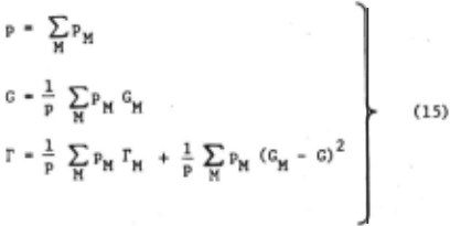
For each match combination, 11M from (2), PM from (12) or (13), and Po from (14) are used in (1) to compute PM· The GM and rM from (8) and (9) with the greatest probability PM can be used for the transformation parameters G and their covariance matrix r. More accurately, if it is desired to in­ clude all matching possibilities and not just the most probable in the solution, it can be computed as follows:

SEARCH PROCEDURE

With a large number of features, it would be impractical to use all combinations in (1) and (15~ However, because of the exponential function in (11) or (13), most of the PM values (and hence PM values) will be negligibly small, and these terms can be ignored. The problem is to determine which combinations will produce significant magni­ tude in PM without having to compute them all.

The approach used is to select the features in Scene A one at a time and tentatively to match As the bottom level of the search tree is reached, not all of the available information will have been used in computing ~M by the above method. Thus ~M from (16) at the bottom level will act as an upper limit to the value that would have been obtained from (2). This effect causes less prun­ ing to occur than the optimum computation would produce, but it should not result in the rejection of good solutions.

At each level of the search, the complete parameter computation according to (3) through (8) can be computed, including the iterations. However, the result from the parent node in the previous level of the search tree can be used as the initial approximation at this node, so that fewer iterations (perhaps only one) would be need­ ed at each level.

Also, under some conditions the variation in the elements of P1 with respect to G can be ig­ nored. (This is likely to occur if G 0 is accurate.) In such a case the summacions involving P 1 in (5) and (6) can be computed recursively by adaing the terms for a new (Ai,Bj) combination to the total accumulated at the parent node, thus saving time (or a Kalman recursive estimation technique, also called sequential adjustment [B), could be used with slight additional time savings). In such a case, time can be saved also in the computation of PM if (13) is used, by recursively accumulating T -1 the sum of Uij Tij Uij and the product of

(2~)a det (Tij) as new combinations are added. G' in (13) would then be constant (perhaps equal to G 0 ). If G 0 is not accurate, it may be necessary to postpone the use of the recursive method until enough features have been matched to determine G well. (An alternate method of recursively comput­ ing PM is described in [2].)

In order to save time in the search phase, it may be desirable to use less than the full infor­ mation that is available. For example, the fea­ ture vector can be collapsed to a vector with fewer components that capture most of the informa­ tion useful in discrimination and adjustment. This would result in slightly less effective pruning, but the time saved in computing each node may more than make up for this. The approximations of this type that can be made depend upon the application. Some are discussed for one case in [2].

In any case, the solution at the bottom level can be used as an initial approximation for one or more iterations with the full computation descri­ bed in the previous section, using those combina­ tions that have not been pruned because of small probability.

EXAMPLE

As mentioned in the Introduction, one possi­ ble application for the method described in this paper is the matching of scene descriptions pro­ duced by the object finder described in [2] and [4]. Such an example will now be presented.

A stereo pair of pictures (each about 100 by 100) taken by the Viking Lander 1 on the surface of Mars was used as the input to processing [2] consisting of stereo depth mapping, a ground find­ er, and the object finder. Figures 1 and 2 show the results when height thresholds of 5 centimetersand 3 centimeters, respectively, were used in the ob­ ject finder. These figures show the ellipsoidal objects (approximating the rocks) projected into the left picture. (The large rock in the center is about 3.5 meters from the cameras and is about 0.3 meters long.) Each ellipsoid represents a feature to be used in the matching process. Arbitrarily a&­ signed feature numbers are shown in the figures. It can be seen that more objects were detected in Fig­ ure 2 than in Figure 1 and that for those objects detected in both cases the ellipsoids are slightly different. Thus two different descriptions of the same scene are available for illustrating the oper­ ation of the matcher. (The poor f . it to the upper right rock was caused by the fact that the background behind it was outside of the right picture, as explained in [2]. The white blob is an artifact of the picture-taking process.)

Although the object finder produces nine para­ meters to define each ellipsoid, only three para­ meters were used here in the matching for sim­ plicity, consisting of the two components of hori­ zontal position and the size. These three parame­ ters formed the feature vector X, and the corres­ ponding three-by-three covariance matrix ~ was de­ rived from the nine-by-nine covariance matrix pro­ duced by the object finder. As a further simplifi­ cation, the covariances of size with position were ignored. The vector G of parameters to be adjust­ ed consisted of the two components of horizontal translation, rotation in the horizontal plane, and scale factor. Translation was completely free to be adjusted (in effect the a priori values had in­ finite standard deviation), the a priori value for rotation wns zero with a standard deviation of 1°, and the a priori value of scale ~actor was unity with a standard deviation of 0.01. The b values, representing the probability of detection of a fea­ ture, were made a function the ellipsoid size,var~ ing from zero for zero size up to 0.9 for a very large object. Po was set to 0.5. This information was used in a version of the matching algorithm ~ plemented for this application and described in de­ tail in [2). The probability threshold for pruning was 0.001 (divided by the number of nodes at this level to obtain an absolute threshold). (This is quite tolerant; in practice a larger threshold may be desirable to reduce the search.) Some prelimin­ ary crude pruning is included in this implementa­ tion. If the discrepancies from (3} are so large compared to the covariance matrix from (4) t-hat it is obvious that this node will be pruned, the further computations for this combination are omitted and thus this node does not appear in Figures 3 and 4. No final adjustment at the bottom level of the search tree was done.

Figure 3 shows the results of using the data in Figure 1 as Scene A and the data in Figure 2 as Scene B. The search tree is shown. The num­ bers at the left followed by colons are the fea­ ture numbers in Scene A. The other numbers on the same line are the feature numbers in Scene B for the features being matched to this feature in Scene A. Zero means that this feature in Scene A is left unmatched. The numbers just below the Scene B feature numbers represent the a posteriori probabilities computed for this match so far. To save space the negative of the common logarithm of the probability, truncated to an integer, is shown. Below the search tree the final results are shown for the most probable match, with computed stan­ dard deviations. Note that the probability is close to 1, whereas the a priori probability was only~. This illustrates the fact that, when the features contain enough information to determine the match well, the a priori probabilities have little effect, as long as they are reasonable. Also note that the standard deviation of the scale fac­ tor is not much less than the input value of 0.01, which means that the solution was not able to add much information about the scale factor. (Since the two scenes were both from the same actual scene and same camera position, the true values of translation and rotation are zero, and the true value of scale factor is unity.)

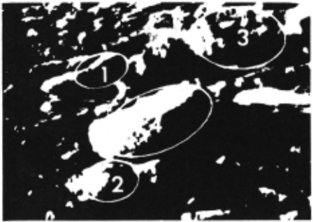
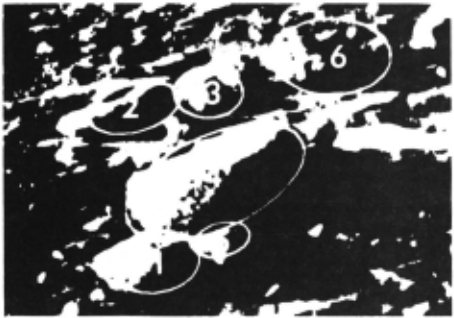
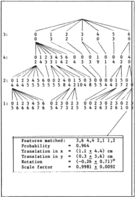
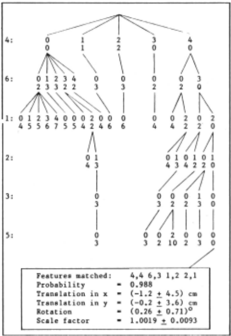
Figure 4. Match of scene in Fig. 2 to scene in Fig. 1.

Figure 4 similarly shows the results of doing the match with the scenes interchanged, so that Figure 2 now represents Scene A and Figure 1 repr~ sents Scene B. Even though the search tree is quite different, the final results are almost the same. (The two final results would agree even better if a complete solution were done at the bottom level of the search tree, since the same features were matched.) Of course, since the scenes have been interchanged, the translation and rotation have changed sign and the scale factor has been inverted.

In this example, only the two horizontal tran­ slation parameters were free to be adjusted by large amounts. Therefore, after the first level, the search tree stopped growing rapidly, because one feature match in two dimensions suffices to determine two translation parameters. If the a priori values of rotation and scale factor had been very uncertain also, the rapid growth would have continued to the second level, because two features matches in two dimensions are required to determine four parameters. However, the rate of growth in general would be less than exponential because of the decreasing computed probabilities of combined incorrect matches, based on local evi­ dence (here only size). If more information (perhaps shape) had been included in the feature vector, the growth might have been less rapid, be­ cause better discrimination against incorrect in­ dividual feature matches would have been possible. Also, a higher probability threshold would reduce the growth. It can be seen that in Figure 3 three of the seven matches at the first level have a probability less than 0.01 and in Figure 4 one of the five does.

After the level of rapid growth discussed above, there is still some growth in the search tree caused by uncertainty in the position of the features. However, most of the growth at these level is caused by leaving the features in Scene A unmatched (indicated by zeros for feature num­ bers in Scene B). As more objects are left erro­ neously unmatched, the probability of these com­ binations becomes quite small at the lower levels of the tree, and they eventually are pruned.