
Object Detection and Measurement Using Stereo Vision
Proceedings of the Sixth International Joint Conference on Artificial Intelligence. .
© 1979 International Joint Conferences on Artificial Intelligence
Abstract
A method of detecting and measuring objects for the purpose of representing three-dimensional outdoor scenes, using data such as that obtained from stereo vision or from a scanning laser rangertnder, Is described. Objects are approximated by ellipsoids. Segmentation of the objects from the background and from each other Is done by finding the ground surface, forming a preliminary segmentation by clustering the points above the ground by more than a threshold, fitting ellipsoids to match these clusters and to avoid obscuring the other points, and adjusting the clusters according to the fits. The method Is designed to produce results useful for obstacle avoidance and navigation In an exploring vehicle, such as a Mars rover. An example il given showing results obtained from a stereo pair of pictures of Mars from the Viking Lander.
- Oennery, D.B. •A Stereo Vision System for an Autonomous Vehicle: In Proc. IJCAI-'17. MIT, Cambridge, Mass., August 1977, pp. 5'16-582. IJCAI
- Nevatla, R. Be Binford, T.O. "Description and Recognition of Curved Objects; Artlf. lnttll. Vol. 8, February 1977, pp. 77-98.
- Hohn, F.E. Eltmtntar' Matrl~ Alg1bra (Third Edition). The MacMlllan Company, 1973.
- Zucker, S.W. •Relaxation Labelling and the Reduction of Local Ambiguities; In Proc. Tlaird International Joint Conf. on Pattern Recognition. San Diego, Calif., November 1976, pp. 852-861.
- Duda, R. Be Hart, P. Pattern R~eognitton and Sc1n1 Anal,sts. Wiley, 1973.
- Bard, Y. Nonllntar Paramtttr Estimation. Academic Press, 197i.
- Graybill, F.A. An lntroduttlon to Ltn1ar Stattsttcal Modtls, Volume I. McCiraw-Hlll Book Company, 1961.
References were extracted automatically from the PDF and may contain errors.
Full text extracted automatically from the PDF; figures, tables and equations may differ. The PDF is the version of record.
1. Introduction
In a previous paper [ ll a stereo vision system and Its possible use In an exploring vehicle wu described. This paper describes further work towards a complete system for an exploring vehicle, specifically, the use of three-dimensional data for the detection of objects and the measurement of their position, size, and approximate shape. Although the three-dimensional data could be obtained from a laser rangefinder, the object detector is designed to be tolerant of errors In this data, such u mistakes produced by Incorrect matches In stereo vision data and poor accuracy of
distances from stereo.
Many approaches are possible In describing the shapes of objects. For example, generalized cones [2] can be used to describe complicated objects. However, in 10111e cases the resolution of the data Is Insufficient to produce detailed Information about the shape. In other cases, the objects are so Irregular as to make such detailed descriptions very difficult. However, In such cases information about the position and size and some crude Information about the shape may still be quite useful. For example, for obstacle avoidance In a roving vehicle, this sort of Information Is adequate. Furthermore, this sort of Information for each object In a large scene containing many objects amounts to quite detailed Information concerning the whole scene, and thus it would be useful for navigation.
· This work was performed under NASA contract NASW-2916 and the Defense Advanced Research Projects Agency contract MD A 90S. 76-C0206.
For these reasons. and because of its convenient mathematical properties, here each object will be approximated by an ellipsoid. By "object" we do not necessarily mean an aC!tual physical object, but merely a portion of the scene that can be reasonably approximated by an ellipsoid. Thus, If we use as an example a vehicle exploring Mars, an object may be a single rock on the Martian surface, two or more adjacent rocks, or merely a bump In the ground. Also, an L-shaped physical object might be represented as two objects.
This ellipsoidal representation should be quite appropriate for representing rocks on Mars, because rocks probably tend to resemble more nearly ellipsoids than any other simple shape. However, It could also be used to represent cars In a parking lot or trees In a field, for example, especially in aerial photographs where the resolution may be poor compared to the size of the objects, and In other cases where precise object description or recognition is not necessary but rather an overall description of the scene is desired.
The stereo vision processing or laser rangefinder results in data representing the three·dimensional position of a large number of points distributed over the scene. The first step In the processing of this three-dimensional data is to find the ground surface. A method of doing this was previously described [ J]. In general, an entire scene would be partitioned Into small areu, In each of which the ground would be approximated by a plane or paraboloid. Then points which are above the ground by a sufficient amount (depending on the computed accuracy of the points, the roughness of the ground, and the minimum size of object that Is of Interest) are candidates for points on objects.
These above-ground points are clustered to produce preliminary groupings of points which correspond roughly to objects. An ellipsoid Is fit to each cluster by first computing an initial approximation based upon the moments of the points In the cluster and then iterating a weighted nonlinear least-squares adjustment to fit the ellipsoids to these points and to avoid obscuring other points. Then, according to the relative positions of the ellipsoids and points, clusters can be broken or merged, and the process repeats until the apparently best segmentation Is found. Each of these steps will be described In the following sections.
The object detection and measurement process as described here uses only the three-dimensional position Information. The brightness Information Is discarded after the stereo processing. However, a more complete system would use both types of information. Perhaps an edge detector could be applied to the brightness data In the regions near the outlines of the ellipsoids in order to refine the boundaries of the objects, for example.
Matrix notation will be used throughout this paper. Matrices will be denoted by capital letters. The transpose of a matrix A will be denoted by AT, and the inverse of A will be denoted by A -1. The trace of a square matrix A (sum of the diagonal elements, which Is equal to the sum of the eigenvalues) will be denoted by tr(A). A vector in three-dimensional space will be represented by a S..by-1 matrix containing the Cartesian coordinates, usually denoted by X with an appropriate subscript. (Hohn [S) provides a good text on matrix algebra.)
2. Preliminary Clustering
Once the ground surface has been determined, all points that are above this surface by more than a threshold are clustered to form an Initial approximation to the segmentation of the scene into objects.
Various clustering techniques could be used here. One possibility Is a relaxation method, such as Zucker's [i). However, at present, the clustering is done by using the minimal spanning tree of the points. (The minimal spanning tree Is the tree connecting all of the points such that the sum of the edges Is minimum.) This Is computed by using the nearest neighbor algorithm [!il (The length of the edges of the tree is defined here as the three-dimensional Euclidean distance between the points.) Then the tree Is broken at every edge whose length is greater than twice the average length of the adjacent edges [!il Howe_ver, a minimum length for an edge to be broken (related to the resolution of the data) is specified, so that the method will not be overly sensitive to local fluctations in the data. Also, a maximum can be specified, beyond which all edges are broken.
S. Initial Approximations to Ellipsoids
Since each ellipsoid will be fit to a cluster of points by an Iterative process, an initial approximation Is needed. A good approximation Increases the likelihood of convergence, decreases the number of Iterations required, and can be used as the result In case the Iterations do not converge. This initial approximation is obtained from the three-dimensional moments, through the second order, of the points In the cluster.
An ellipsoid can be represented by the following matrix equation:
where X Is a vector of the three-dimensional coordinates of any point on the surface of the ellipsoid, Xc similarly Is the position of the center of the ellipsoid, and W is a positive-definite symmetrical S.by-S matrix. (See, for example, Hohn [Sl) Let M denote the inverse of W. (The square roots of the eigenvalues of M are the lengths of the semi-axes of the ellipsoid.) The relationship between the computed moments and the matrices Xc and M depends on the distribution of points over the ellipsoid. If the object has been viewed from a single point, we will have points distributed nonuniformly over half of the surface. (Actually slightly less than half will be seen because of perspective. Also, in stereo vision, both cameras must see each point, so that with a single pair of cameras only the common area seen from both camera positions will appear. These two effects will be neglected below, however.)
We assume here that the object Is seen from a single viewpoint by a raster scanning device which produces points distributed uniformly in the Image plane. Such a device might be a scanning laser rangefinder or an area-based stereo system. Actually, because of missing points, the distribution wlll not be uniform. It would be possible to estimate the actual distribution by computing higher-order moments, but this might be overly sensitive to randomness in the distribution or an Inadequate density of points, so it is not attempted here. As an approximation, we assume an orthogonal projection Instead of a central projection. Let X, denote the vector of normalized first moments (centroid) and MA denote the matrix of second moments about X 1 obtained with this distribution, and let X 0 denote the position of the camera.
The relationship connecting X, and M, to Xc and M can be derived by first considering the case of a sphere of radius r. A little integration shows that in this case the eigenvalue of M 1 corresponding to the eigenvector X 0 -Xc is r 2 /18, the other two eigenvalues are both r 2 /i, and X 1 Is Xc plus 2r/S times the unit vector In the X 0 -Xc direction. All three eigenvalues of M should be r 2 in this case. An ellipsoid can be considered to be a distorted sphere (using stretching and skew distortions). Thus the ellipsoid can be considered to be stretched In the various directions by the amount given by the square roots of the ratios of the above eigenvalues, but in computing the displacement of the center, instead of r the distance from Xc towards X 0 to the ellipsoid surface must be used. Thus the displacement of the center Is the vector
2(X 0 -Xc)/3 divided by the scalar ~J<X0Xc)TW(X0·Xc>· Since Xc· X 1 , and X 0 are colinear, Xc can be replaced by X 1 without changing the value of this ratio. Also, W (·M- 1 ) can be replaced by M,- 1 118 In this expression, because of the stretching discussed above. Thus Xc can be computed from X 1 by translating by this amount. To compute M, we can take 4 times M 1 to account for the factor of 4 In two dimensions, but this leaves 14 out of the factor of 18 by which we need to stretch the moments In the direction toward the camera. This extra amount can be added by adding li times the moment produced by a fictltous point at the Intersection of the X 1 -to-X 0 line and the surface of the ellipsoid corresponding to M 1 . In order to keep the ellipsoid to a reasonble shape when there are not enough points to determine It well, M as obtained above is averaged with a scalar matrix whose diagonal elements are s (which represents a sphere of radius .JS>. with the average weighted so that the sphere represents four additional points in the moment computation. The value of s is determined so that it Is the average of the two components of the second moments at right angles to X 0 -X 1 , but limited by the average of all three components (the three eigenvalues), including the effect of lot times the effect of the fictitious point, u above, u an upper limit, and excluding this effect, u a lower limit. This avoids putting undue weight on the X 0 -X 1 dimension when the ellipsoid Is long In this direction, since this dimension Is less reliable because of the factor of 18 compression.
By combining the above Information, the computation of the lnltlal approximation can be expressed u follows:
where XP represents any point in the cluster, n Is the number of points In the cluster, the summations are over these points, and I Is the 3-by-3 identity matrix.
4. Iterative Solution for Ellipsoids
The adjustment of the ellipsoids Is done by a modified least-squares approach. Each ellipsoid is adjusted so as to minimize the weighted sum of the squares of two kinds of discrepancies: the amounts by which the points (usually points In the cluster being fit) miss lying in surface of the ellipsoid, and the amounts by which the ellipsoid hides any points as seen from the camera position. (In the latter case, the discrepancies actually should be considered separately for each camera that sees the point in question. However, for narrow-angle stereo we use as a reasonable approximation the assumption that the "camera" is at the midpoint of the stereo baseline.) Including the second kind of discrepancy is useful In helping to determine the size and shape of the object when the points on the object itself do not contain sufficient information. Also included in the weighted sum of squares to be minimized are a priori terms which tend to force the ellipsoid by default to become a sphere near the ground when the points do not constrain it well.
The first kind of discrepancy above optimally should be defined as the length of the normal from the point in question to the surface of the elllpsoid. However, computing this requires solving a sixth-degree equation. Therefore, as an expedient the distance between the point and the surface along a straight line from the center of the ellipsoid to the point Is used instead. In order to be consistent with this definition, the second kind of discrepancy is defined as follows. The midpoint of the two intersections of the surface of the ellipsoid with a line from the camera to 'the point is first found. Then the discrepancy of the first kind Is computed for this midpoint. Both kinds of discrepancies are illustrated In Figures I and 2.
Now we must consider exactly for which points which kind of discrepancy is computed. There are five regions of space to consider, according to whether the point is to the side of the ellipsoid as seen from the camera (that is, the line through the camera postion and the point does not intersect the ellipsoid), is in front of the ellipsoid as seen from the camera, Is Inside the front portion of the ellipsoid (In front of the surface of midpoints as defined above), is inside the back portion of the ellipsoid, or is behind the ellipsoid. Also, there are two kinds of points to consider, according to whether or not the point is In the cluster which Is assumed to correspond to this object. This produces ten combinations in all, which are illustrated in Figures I and 2. They divide into four categories.
First, If the point is not in the cluster and is either in front of the ellipsoid or Is to the side, there is no discrepancy and this point is not included In the computations.
Second, if the point is in the cluster and is either in front, Inside the front half, or to the side, or if the point is not In the cluster and Is inside the front half, the first kind of discrepancy Is used.
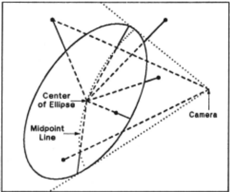
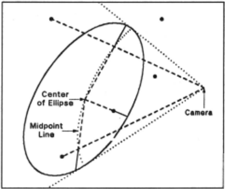
Third, If the point is not In the cluster and is behind the ellipsoid, or if either kind of point Is Inside the back half, the second kind of discrepancy Is used.
Fourth, if the point is In the cluster and is behind the the ellipsoid, both kinds of discrepancies are used, and the point acts as two points In the computations. This Is because there are two separate components of error in this case: the object does not extend enough on the side to hide the point, but It apparently bulges out In back (relative to the ellipsoid) to Include the point.
In order to derive the mathematics for dividing space Into the above five regions, consider the equation for the ellipsoid, as previously stated,
and the equation of a straight line through the camera position X 0 and the point In question XP' in parametric form,
These can be combined to produce
the roots of which determine the Intersections of the line and ellipsoid. This equation Is equivalent to
The roots of the above equation In u determine the r~ion of space In which XP lies. If the roots are Imaginary (b -iac < 0), the point Is to the side of the ellipsoid. If the average of the two roots (-b/2a) Is positive, the point Is In front of the midpoint surface, If negative, It is behind the surface. If the roots are real, the point is In front of, behind, or inside the ellipsoid according to whether both roots are greater than unity, both roots are less than unity, or unity lies between the roots, respectively. Alternatively, we can use the fact that the point is outside of the ellipsoid If and only If (Xp-Xc)TW(Xp·Xc) > 1.
The discrepancy of the first kind Is
In order to compute the discrepancy of the second kind, the midpoint of the Intersections of the camera-point line with the ellipsoid is first obtained as follows:
Then the discrepancy of the second kind is
Because there may be erroneous points in the data, points
where which have large discrepancies relative to the site of the ellipsoid are given less weight in the solution. The weighting function used Is
where X represents XP or Xu for discrepancies of the first or second kinds, respectively, and cr Is the component of standard deviation of measurement errors in XP propagated Into the discrepancy. (If these are unknown, cr can be zero.) Thus the dimensionless quantity to be minimized (by adjusting Xc and W) Is l:WE 1 , plus some additional terms for a priori values yet to be discussed. However, this quantity is minimized only with respect to the effects of Xc and W acting through E and not their effects through w. In order to solve the above nonlinear problem, the Gauss method [6] is used. This method Is equivalent to using the partial derivatives of the discrepancies to approximate the nonlinear problem by a linear statistical model [71 solving the linear problem, and Iterating this process until it converges.
On any one Iteration the following is done. The current values of Xc and W are used to compute for each point the value of E as define above and the 1-by-9 matrix P, which consists of the partial derivatives of E with respect to the three elements of Xc and the six unique elements of W. (W Is symmetrical.) The following summations over all of the points are computed, In which each point In the first category above Is not used, each point In the second or third categories appears once, and each point in the fourth category appears twice:
(Ho and c 0 are used for the a priori values yet to be discussed.) Then the 9-by-1 matrix of corrections Is
where v Is a factor used to Improve convergence because of the very nonlinear nature of the problem. (Currently v · 0.5 on early Iterations, but v · I after a test indicates that this will produce more rapid convergence.) The elements of D are subtracted from the corresponding elements of Xc and W to obtain the Improved approximations for the next Iteration.
Now the a priori values will be discussed. In some cases the points affecting the ellipsoid will be insufficient in number or insufficiently distributed to determine all parameters of the ellipsoid very well. It is therefore desirable to have a priori values for some of the parameters with appropriate weight in the solution to constrain them to reasonable default values when the points do not contain sufficient Information. When there Is ample information In the points, the a priori values will have very little effect because of their small weight. The a priori values currently used are the ground surface height directly under Xc for the vertical component of Xc· with weight 0.1 /tr(M), equality for the diagonal elements of W, with weight tr(M)Z/10, and zero for the off-diagonal elements of W, with weight tr(M)2/IO, where M · w-1. (Including tr(M) as shown scales things correctly so that the solution is invariant under a scale factor change.) The effect of the W terms is to try to force the ellipsoid into a spherical shape. These a frriori terms are put into the solution in the following way. The diagonal element of Ho corresponding to the vertical component of Xc is 0.1/tr(M), the three diagonal elements corresponding to the off-diagonal elements of W are each tr(M)2/IO, and the 3-by-3 submatrix on the diagonal of Ho in the position corresponding to the diagonal elements of W consists of 2/3 on its main diagonal and -1/3 elsewhere multiplied by tr(M)2/IO. All other elements of the 9-by-9 matrix Ho are zero. Then
where G is a column matrix of the current values of Xc and W, arranged as in D, with the height of the ground directly under the center of the ellipsoid subtracted from the element of G corresponding to the vertical component of Xc. H0 and C0 are used In the summations for H and C as previously shown.
5. Breaking and Merging Clusters
Because the preliminary clustering is dependent on local information, it may not produce the best segmentation based on more global information. Therefore, after ellipsoids have been fit to all of the preliminary clusters, these clusters may be tentatively broken into smaller clusters and merged into larger clusters, new ellipsoids are fit to these clusters by the same process previously described, and a decision on whether to keep or reject each of these actions is made based on the goodness of fit of the ellipsoids to the points.
In order to decide where to break a cluster, for each edge in the portion of the original minimal spanning tree which connects this cluster the quantity ;\( J.p) is computed, where;\ is the length of the edge and p is the minimum of
J<xp.xJI'w(Xp-Xc) for the two points connected by the edge. Then the cluster is tentatively broken at the edge for which this quantity Is maximum, of all such edges such that each new cluster form~d has at least four points at least one of which has (X -Xi W(X p·Xc) > I (that is, it is outside the old ellipsoid). This process tends to break the cluster at places furthest inside the ellipsoid, but connecting points that are outside the ellipsoid. If this new clustering Is accepted by the criteria described below, the process repeats on the new clusters.
After the above breaking process is, finished, any two clusters are tentatively merged If (X 1 ·Xi W(X 1 ·Xc) < i for either cluster, where X 1 Is Xc for the other cluster, provided that these two clusters were not previously one cluster before breaking. If there is competition for the merging, the cluster pair with the minimum value for this quantity Is merged first. Ir a merger Is accepted, further mergers can take place on these clusters by this same process.
The criteria for accepting two clusters or one that resulted from a tentative break or merger are as follows. If (X 1 -Xc)TW(Xa-Xc) < I for either small cluster, where Xa is Xc for the other small cluster (that Is, the center of one ellipsoid Is inside the other ellipsoid), the single cluster is chosen. Otherwise, the following quantity is computed for each of the three ellipsoids:
where E and w are the discrepancies and weights from the last Iteration, as defined in the previous section, and n is the number of points In the cluster corresponding to this ellipsoid. (If the Initial approximation is used as the result, E and w are obtained from the first iteration, and the denominator is n instead of n-S.) Then the two small clusters are chosen if the sum of their two values of q is less than the value of q for the single cluster. Otherwise, the single cluster Is chosen.
6. Results
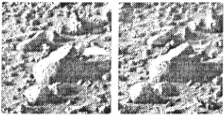
Fig. S shows a stereo pair of pictures taken from the Viking Lander I on the surface of Mars. Each picture is 256 pixels by 256 pixels. The pixel spacing is 0.04 degrees in azimuth and elevation. (Thus the field of view is about 10 degrees.) The azimuth and elevation from the left camera to the center of the picture are about 18 degrees and -20 degrees, respectively, relative to the camera positions. The two cameras are 0.8187 meters apart. The distances to the points In the scene range from about S meters to about i.!i meters.
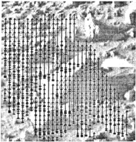
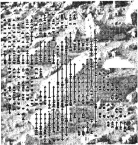
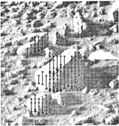
Fig. i shows the left picture enlarged, with arrows indicating the points found by the stereo processing. The point of each arrow Is at the center of an eight-pixel-square window which was matched to a corresponding area In the other picture. (Thus the resolution of the reduced stereo data is 0.32 degrees In azimuth and elevation.) The arrows are dropped perpendicularly from the point In three-dimensional space computed for this point to a nominally horizontal reference plane J.!i meters below the cameras, with the base of the arrows on this plane, and are then projected Into the picture. Fig. !i shows the same data as Fig. i except that the bases of the arrows rest on a ground plane computed from this data by the ground surface finder. Fig. 6 is the same as Fig. !i except that It shows only points computed to be at least !i centimeters above the ground surface.
The 5-centimeter height threshold was used for selecting the points to cluster In the object finder. The minimum distance for breaking the minimal spanning tree to form the Initial clusters was also 5 centimeters, and the maximum distance for connecting points was 20 centimeters. (Using zero and Infinity for thl.s minimum and maximum produced a sightly different Initial clustering but identical final results.)
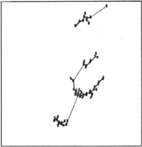
Fig. 7 shows the points In Fig. 6 In a nominally vertical orthogonal projection (perpendicular to the reference plane). The figure covers an area one meter by one meter. The symbol for each point represents height In centlmenters above the ground plane, with the letters A, B, C, etc. representing the values 10, II, 12, etc. The points are connected to show the minimal spanning trees that were computed. Solid lines connect points within each Initial cluster.
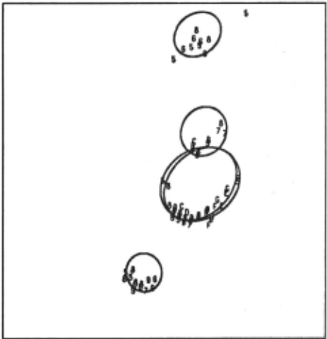
Flaure B. Ellipsoids fit to lnltiel clusters.
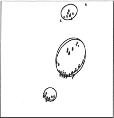
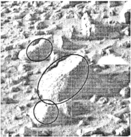
Fig. 8 shows the ellipsoids that were fit to the initial clusters. Each ellipsoid Is represented by two ellipses. One ellipse is the orthogonal projection of the ellipsoid onto the reference plane. The other ellipse Is the Intersection of the ellipsoid with a plane through the center of the ellipsoid and parallel to the reference plane. Only the clustered points are shown here, as in Fig. 7. However, as previously described, any of the points shown In Fig. i may have been involved in the adjustment of the ellipsoids. Remember that the fit Is done In three dimensions, whereas Fig. 8 shows a two-dimensional pro jectlon.
Fig. 9 shows In the same way the results of the breaking and merging operations. The two clusters in the center (corresponding to the large rock in the center of the pictures) were merged Into one, and a new ellipsoid Is shown for this cluster. The other clusters were not changed.
These results were projected into the left picture to produce Fig. 10. The outline of the ellipsoids as they would be seen from the left camera are superimposed on the picture. The lengths of the principal axes of the large ellipsoid In the center are 36.5, 30.5, and 19.8 centimeters.
Acknowledgment
The Mars pictures were supplied by Elliott Levlnthal and Sidney Liebes of the Viking Lander Imaging Team.
@inproceedings{ijcai1979p71,
  title     = {Object Detection and Measurement Using Stereo Vision},
  author    = {Gennery, Donald B.},
  booktitle = {Proceedings of the Sixth International Joint Conference on
               Artificial Intelligence, {IJCAI-79}},
  publisher = {International Joint Conferences on Artificial Intelligence},
  editor    = {Bruce G. Buchanan},
  year      = {1979},
  month     = {8},
  url       = {https://ijcai.org/proceedings/1979/71},
}
TY - CPAPER TI - Object Detection and Measurement Using Stereo Vision AU - Gennery, Donald B. T2 - Proceedings of the Sixth International Joint Conference on Artificial Intelligence, IJCAI-79 PB - International Joint Conferences on Artificial Intelligence PY - 1979 UR - https://ijcai.org/proceedings/1979/71 ER -Copied
Machine-readable versions of this paper, for tools and AI agents:





