A Theory for the Complete Mechanization of a GPS-Type Problem Solver

1. Introduction

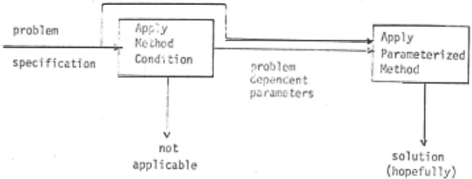
According to our view of mechanical problem solving, there are a number of different problem solving methods each of which has problem depen­ dent parameters. For each method there is a con­ dition which specifies the properties the parame­ ters should have in order for the method to "work". Hence, we view problem solving as the two phase process shown in Figure 1. In the first phase, the method's condition is used to generate "good" parameters for the method. The input to this phase is the problem specification, since the parameters are usually problem dependent. The output is either good parameters or an indication that this method should not be used on the given problem. The second phase attempts to solve the problem (as specified at the input to the first phas.e) using the method with the parameters gener­ ated in the first phase. Of course, there is a oicture like Fi~ure 1 for each method, and if the first method is not applicable, we merely move on to the next method and attempt to use it.

So far, all the methods studied this way [Co­ ray(l970), Ernst(l969), Banerji(l971)] seem to depend on the recognition of certain attributes of the problem states which remain invariant under some of the moves. We have previously published two reports on the design and implementation of a program which would isolate some of these attri­ butes on the basis of the problem description [Ernst et al(l974), Oyen(l975)].

Our present effort deals with the combination of the invariant properties to yield the Connec­ tion Table of GPS [Newell & Simon(l963), Ernst & Newell.(l969)]. Our efforts in using our previous theory [Ernst(l969)] for the purpose of mechaniz­ ing the heuristic were not successful, because a difference (good or bad) was a binary relation between states and sets of states, i.e., a subset of S x 2S where S is the set of problem states, which is a complicated concept.

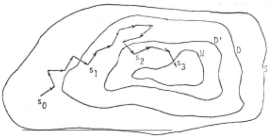
In an attempt to simplify matters we said, "What if a difference were just a set of states?" In this case, a state s possesses difference D, if s t D. With this simple view we can visualize GPS's strategy as follows (Figure 2).

S is the set of all states. W is the set of goal states: W c D' c D c S, and s 0 is the initial state. GPS would attempt to solve the problem as follows:

1. Find a path from s 0 to some state s1 E D.
2. Find a path from s 1 to some state s2 E D' but the path must be entirely inside D.
3. Find a path from s2 to some state s3 E W but the path must be entirely inside D'.

In step 1 GPS is removing the most difficult dif­ ference D. In step 2 the second most difficult difference is being removed without reintroducing D. The easiest difference W is being removed in step 3 without reintroducing either D or D'.

A point ought to be made here about the orig­ inal GPS which was a somewhat more general device than the one we are describing here in that, while removing an easier difference, a more dif­ ficult difference could get reintroduced. The only search pruning involved in this general case was that involved in the relevance of moves to differences (vide ultra). The extra constraint we have introduced here (and one which also char­ acterizes our previous work [Ernst(l969)]) con­ strains the search for greater efficiency, while at the same time it neglects a certain class of solutions. Our present analysis follows the same line.

It is probably somewhat counterintuitive that the most difficult difference contains all of the other differences as subsets. One would normally think that the larger the set of states, the eas­ ier it would be to "get" inside of it. Also, one does not normally think of Was a difference. But this somewhat unintuitive picture works quite well.

Consider, for example the Fool's Disk problem. Figure 3 gives the initial state of the Fool's Disk problem, in which there are 4 concentric disks each containing 8 numbers. These numbers line up so as to form 8 columns radiating from the center of the disks. A move consists of ro­ tating one of the disks ind~pendently of the oth­ ers. The desired state is one in which each of the 8 radial columns sums to 12.

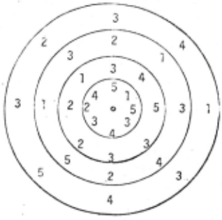
This problem fits the above picture exactly. D' is the set of states in which each diameter _sums to 24, whileD is the set of states in which the sum of theN, E, S, and W radii is 48. To keep the path from s1 to s 2 in D, GPS only consid­ ers moves which rotate disks 90°. To get from s1 to s3, GPS rotates disks by 180° only.

One might be disturbed that each difference contains all of the easier differences. This is not a difficulty, because any set of differences not possessing this property can be converted to differences which have this property. (In fact, . our theory [Banerji &. Ernst(l977)] does not re­ quire this "nesting" of differences.) Consider, for example, the 3 disk Tower of Hanoi in which we 'are trying to move all disks to peg P 3 . Let Di be the set of states in which disk i is on P3 where disk 3 is the largest disk. Then, one might think ·of using D 1 , D 2 , and D 3 as differences for this problem. These are essentially the differences that-.were given -to: GPS for - this· problem. Certain­ ly these sets are not perfectly nested. However, this set of differences can be converted to the above picture by intersecting them together, i.e., D = D 3 , D' = D 3 n D 2 , and W = D 3 n D 2 n D 1 .

A more disturbing feature of this set of dif­ ferences is that they are only useful when the set of desired states is W. In the original GPS (as well as in our previous work) the same set of dif­ ferences served to characterize all subgoals - including "make such and such a move applicable." This is not the case anymore. If, for example, the set of desired states is the domain of the operator which moves disk 3 from P 1 to P 3 , the Di seems to be a useless set of differences. The difficulty is that we have "built" W into the dif­ ferences. We did this on purpose to simplify the differences to allow mechanization. Our original theory had differences as binary relations bet­ ween states and sets of states. If we specify the latter to be W, then we are left with a mo­ nadic relation on states which is just a set of statas. But how are we going to accommodate goals other than W?

The key to answering this question is that not only W but also the domains of operators can be the goals of subproblems. Since the number of op­ erators.is usually quite_small, we will use a different set of differences for the domain of each operator being the goal of a subproblem.

These modifications were introduced in our theory of GPS to make it easier for person or machine to discover "good" differences. An added advantage of the modified GPS is that it can eas­ ily handle problems in which the sets of differ­ ences for subproblems with different desired states are truly different.

The above discussions will, we hope, serve as a motivation for the changes we have introduced in the theory. We do not plan to give a formal counterpart to these motivations or exhibit a for­ mal connection between the old and the new theories. Instead, we shall exhibit and motivate the new theory ab initio so that readers unac­ quainted with our previous work will find the discussion self-contained. We shall, of course, assume that the . rea~P.r has "ha.d former acquain­ tance with GPS [Ernst & Newell(l969)].

In the next section we give a formal defini­ tion of good differences. This is followed by an example of good differences and how they are used by GPS. Section 4 characterizes the c lass of -so­ lutions that GPS can find given the kind of dif­ ferences described in Section 2.

2. Definition of Good Differences

Since GPS builds its solution to a problem by setting up subproblems, we cannot build this theo­ ry by defining what a problem is but rather by de­ fining a larger structure in which a class of sub­ problems can be embedded. Also, this structure should contain the concepts which reflect the idea of differences and the connection table. We shall call this structure the problem domain, "domain" for short. As in the previous models, we start with a set S of states and a subset W of S, con­ sisting of winning states. We also have a set G of partial functions (mapping subsets of S into S) which we shall call moves or operators. If f E G is a move, we shall denote by S£ its domain of de­ finition, i.e., states where f is an applicable move. Since subgoals in GPS have the form "make move £·applicable," these Sf, for various members f of G, serve as winning sets for subproblems just as W serves for a problem. The class of all these sets (W and Sf for various f) we shall call X. For each set in this class we also define the dif­ ferences which allow GPS to work on them. That is, for each T £ X (T being either W or Sf for some f £G) we define a class of sets T1, T 2 , T 3 ... Tn with the property that T 1 n T 2 n ·.· Tn = T. The actual number n of specified differences of course depends on the set T chosen. So, instead of writing n we shall write n(T) when there is any doubt as to which subproblem we are talking about. Also, for reasons of convenience of dis­ cussion we shall often give the name To to T and

· call S itself, Tn(T)+l·

It may be appropriate at this point to point out that the Ti catches the idea of difference in that when a state s i Ti, a difference exists between s and T. The higher i is, the lar.ger the difference is.

The next important concept in GPS, of course, is that of relevance of a move to a difference. The major assumption on which GPS theory is based is that a solution can be obtained by removing the higher ("more difficult") differences before the lower differences and never reintroducing higher differences once they are removed. A dif­ ference is considered higher than others, if few·er moves are available to remove it. Of course, S or Tn(T)+lare the most difficult differences to remove, since no move changes a state to a non­ state. Let Hi s G be the set of moves which, _when applicable, affects the position of the state with respect to Ti. · Instead of making the very strong assumption that moves in Hi bring all states outside Ti into_ Ti' we shall make the more realistic assumption that these moves remove the states from Ti when appiied. This assumption seems "backward" to many, in spite of the fact that in most real problems, relevance of moves does appear that way and was used that way even in the original GPS. In our difference-finding program, a state is characterized by giving the values of certain attributes for the state. A winning state is characterized by specifying that some of the attributes should have specific unique values. To find mechanically that a cer­ tain move is relevant to a certain difference Ti' we test whether the move changes the values of those attributes which characterize Tj.

It is th.is "property-changing" characteriza­ tion for moves which gives relevance the backward appearance. Of the various values to which the attribute can change, only one characterizes the . win states. Hence, it is not to be expected that merely changing the value of a property yields a win value. On the other hand, if it already has a win value, changing it certainly changes it to a non-win value.

Another important characteristic we demand of the moves in Hi (called triangularity of the dif­ ference table in the previous theory) is that Hi does not affect the differences higher than Ti, i.e., is irrelevant to Tj for j > i. Thus, once a state is in Ti, as long as we use moves in Hj with j < i, Ti will not be reintroduced.

This effort shows up nicely in the difference transformation tables of GPS. If we arrange the Ti's from top to bottom in decreasing order of i and the H from left to right in decreasing order, and mark ihe (i,j) cell with a 1 if moves in Hj are relevant to Ti, then the upper right half of the table will be blank. Tables of this nature we call triangular tables, and differences which give rise to triangular tables we call good differences.

We define the maximum difference between T and s, M(s, T), to be i if s i Ti and s E Tj for all j greater than i.

Implicit in the above definitions is an or­ dering of the Ti (and the Hi) which corresponds to the difference ordering of GPS. The most dif­ ficult difference is Tn, while the easiest dif­ ference is T1. GPS's basic problem solving strategy is to work on hard differences first and easy differences last. GPS accomplishes this (as discussed in Section 4) by using the following to guide its search:

• Sl To reduce the maximum difference Ti, use only operators in Hi.
• S2 Suppose a subproblem were generated to reduce difference Ti. Then do not use the operators in Hj, i ~ j ~ n ~ solve the subproblem.

Rule Sl was in our previous theory. Note that there may be many other operators besides Hi which are relevant to Ti because we have placed no con­ ditions on Hj for j > i. Sl causes GPS to ignore such Hj even though some of its operators may be relevant to T i.

The purpose of S2 is to require subproblems to be easier than the problem for which they are created. In our previous theory this was accom­ plished by requiring the differences of a problem to be harder than the differences of its subprob­ lems. This is no longer possible, because we can­ not compare subproblem differences to problem dif­ ferences because they will have different goals and hence different differences. However, S2 can be used, because all differences are reduced by the same operators. Note that S2 is applied re­ cursively. That is, suppose Fl and F2 are the sets of operators according to S2 that cannot be used on subproblems SPl and SP2, respectively. If SP2 is a subproblem of SPl, then GPS will not use any operator in Fl u F2 to solve SP2, because the restrictions on SPl are passed down to all of its subproblems.

3. An Example of Good Differences

The definitions above appear quite formidable and somewhat unlike GPS. A simple example will clarify things. For our example we have chosen that old chestnut about the monkey and the ba­ nanas, a formulation of which is given in Figure 4. We have chosen this example because it has (non-trivial) good differences, subproblems are created in solving it, and it is simple.

One way to formalize the differences above is by positing that there is a separate table of connections for each goal which is either W or the domain of an operator. Figure 5 illustrates Mon­ key and Bananas this way. The l's indicate which operators are relevant to which differences. The O's indicate irrelevance. A move is neither rel­ evant nor irrelevant - we use a question mark. Note that the bottom row heading of each table is just the goal and that each row is a subset of the row above it. Although our theory does not require these properties, they make things easier to visualize as discussed at the beginning of

• s A state is a 3 place vector whose com­ ponents are the monkey's position, the box's position, and. the contents of the monkey's hand.
• w A win is a state in which the bananas are in the monkey's hand.
• G {walk, Climb, Push, Grab}
• Walk The monkey walks to someplace in the room.
• Climb The monkey climbs onto the box, i.e., the monkey's position becomes ONBOX. Climb is applicable only when the mon­ key's position equals t~e box's position.
• Push The monkey pushes the box to some in the room. Push is applicable only when the monkey's position equals the box's position.
• Grab The monkey grabs the bananas. Grab is applicable only when the monkey is on the box, and the box is under the ba­ nanas.

Figure 4

A Formulation of the ~lo r.key and Bananas Proo~em

Section 2.

The row headings are the Ti in the defini­ tions of Section 2, and the column headings are the Hi. The definitions of the Ti and the Hi re­ quire that the tables of connection are triangular in the sense that the main diagonal and all en­ tires above it are 0. In addition, the subdiagon­ al (the diagonal immediately below the main diag­ onal) contains all l's.

Walk is a total function on S, hence its do­ main is S. We do not need a table of connections for such an operator, because a subproblem of get­ ting into its domain will never be created. We included the table of connection for Walk in Fig­ ure 4, because the degenerate case of a defini­ tion often helps one understand the definition.

If a column of an operator is all O's, then that operator will never remove a state from the goal set and will never transform a state outside the goal set into the goal set. An all 0 row in­ dicates that no operator will add or remove a state to the Ti which labels the row.

The above is an example of "difference in­ formation" which satisfies our definition of good in Section 2. The most important feature of the tables in Figure 5 is that the triangularity con­ straint orders the rows (and the columns). This row ordering is the difference ordering - diffi­ cult differences are at the top of a table, and easy differences are at the bottom. Of course, there may be several different row orderings which gives rise to a triangular table, in which case any one of them will satisfy our formal de­ finition of good.

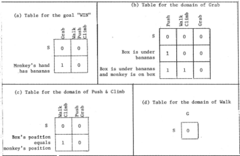
Now we can describe how GPS solves Monkey and Bananas using the difference information in Fig­ ure 5. Suppose that in the initial state so the monkey's hand is empty and the box is not under the bananas. Then the largest difference, M(so,W), is that the monkey's hand is .empty. hence GPS attempts to apply Grab. But so ., Sgrab· hence GPS sets up the subproblem of transform~ng so 1nto Sgrab· but Grab cannot be used in solving the sub­ problem because of rule S2.

To solve the subproblem, GPS attempts to re­ duce the difference that the box is not under the bananas since this is M(so, SGrab>· Hence, GPS attempts to apply Push which is not applicable, and the subproblem of transforming so into Spush is generated, but S2 restricts the solution"of this subproblem .to the operators Walk & Climb. The remaining part of solving this problem is quite straightforward and similar to the way the usual GPS works.

4. Totally-Ordered Solutions

The above discussion raises the question, "Can GPS solve all problems which have a solu­ tion?" The answer is no (which can be shown quite easily), because"the differences, together with rules Sl and S2, prevent GPS from looking at sequences of operators that may be necessary to find a solution. Hence, the question become~, "Can we somehow characterize the class of problems which GPS can solve?" The purpose of this section is t~ show that GPS can solve any problem that has a totally-ordered solution which is our character­ ization of the class of problems that GPS can solve. Intuitively a totally-ordered solution is one in which one never introduces a difference ·more difficult than the current differences at any point in solving the problem. This applies to all subproblems at all levels. We will indicate in Theorem 1 that using rules Sl and S2 with good differences produces the class of totally-ordered solutions.

To exhibit this result we have to give de­ finitions of what a problem is and what a solution is. Given a domain as defined in Section 2, a problem is defined by a state s E S, a subset F of G (the set of moves), and a goal T E X. A solu­ tion of a problem defined by the triple <s·, F, T> is a sequence of moves (fl,····fk), each fi (1 s i s k) being an element of F, and such that sf, ... fi is defined for all i (1 s i s k) and sfl···fk E T.

At this point we invoke the partition Ho(T), Hl(T), ... ,Hn(T)(T) and recall that each fi in the above solution is an element of some Hj(T). This yields a sequence jl, j2, ·.. ,jk of integers such that for each i, fi E Hji(T). Among them will now occur an integer which is greater than all the in­ tegers before it and no less than any element af­ ter it, i.e., the "leftmost peak" below, where we have plotted ji against i.

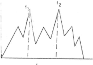
We will initially show that the solution can be interpreted to mean that, at this point, the first effort was made to remove the highest dif­ ference between the goal and the initial state s. The moves before this peak are attempts to make it possible to apply the move used at the peak. This sequence (from the start to the peak i 1 ) will be called the solution to the subproblem, an~ the sequence between it and the end will be called the solution to the pseudoproblem. The rest of the definitions follow from these considerations.

The triple ~ (f1 , ... fi 1 _1), fi 1 ' (fi +l···· fk) > is called the parse of the solution 1 f 1 , ... fk. It is obvious that given a doma in and a solution of any problem <s, F, T>, the parse exists and is unique.

Given the parse as above, we define two problems. The first, which is defined only in the case that i 1 > 1, is

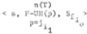
and will be called the subproblem of <s, F, T> corresponding to the solution (f 1 , ·.. fk). The second, which is defined only when i 1 < k, is

and will . be called the pseudo-problem of <s, F, T> corresponding to the solution.

Once again, it is obvio11s that f 1 , ..· fi 1-1 is a solution of the subproblem corresponding to the original solution.

Thus, one can say that any solution can be interpreted, i.e., parsed, to be one in which one seeks to apply moves in I:Im(T) with "the highest m," making ~uch a move applicable by using moves only in H (T) with p < m. However, such an inter­ pretationpcould be given with any ordered parti­ tion, having nothing to do with a difference ordering. The reader will recall that in our orig­ inal definition of a domain the partition on F was so done as to be in keeping with the differ­ ences.

To bring our discussion back to the differ­ ence orderings rather than with the partitions on the moves, we introduce another definition. Given a problem <s, F, T> and a solution (fl·····fk) and a parse, the solution is called totally ordered, if

tii) each subproblem and pseudoproblem has its corresponding solution totally ordered.

Totally ordered solutions are of importance in that they characterize the kind of solution that can be found by the technique used by GPS. So far we have not formally defined this technique. The statement of the following theorem formalizes the technique as well as characterizes solutions that can be found by it. However, the statement of the theorem needs the following definition.

Given a problem <s, F, T> in a domain and a solution f , .·. ,fk for it, the problem-set for this solution consists of the problem and the mem­ bers of the problem set for the solutions to the sub- and pseudo-problem of the original problem, if they exist.

We are now ready to state the major theorem of this paper.

Theorem 1: Given a solution (f 1 , f 2 , ··· fk) of a problem <S, F, T> in a domain, the solution is totally ordered, if and only if for each i (1 ~ i < k), fi is the second element of the par­ se of the solution of some problem <s', F', T'> in the problem set, and fi E Hm(T') implies M(s', T') = m .

Intuitively, this theorem says that, if the solution (f 1 , ... fk) were found by a search process guided by rules Sl and S2, then it is totally or­ dered. In addition, such a search process is ca­ pable of finding any totally ordered solution.

We shall not include the proof, because it is a long "walk along the definitions" given above and needs some more inessential pedentry like transfinite induction (on a finite space at that!).

5. Conclusion

We now have a working program [Goldstein (1977)] which, using invariant attributes of the problem [Oyen(l975)], would construct a set of properties Ti and partitions Hi as given in Sec­ tion 2. These would yield what we have previously called triangular connection tables.

It will be noticed that, as previously warn­ ed, Theorem 1 of Section 4 does not assure us of a solution whenever a triangular difference table exists; one has to be blessed with a totally or­ dered solution - totally ordered by the ordering mechanically or otherwise chosen in the connection table. We have had various problems in which more than one triangular connection table exist, and yet one can prove that some of the connection ta­ bles would not yield a solution. This problem has appeared in other, seemingly closely related, garbs in planning programs for Robots, leading to the work on Non Linear Plans [Sacerdoti(l975)]. The analogous problem in our formalization would be the detection of the nonexistence of totally or­ dered solutions. One approach, that of the detec­ tion of "factorable subproblems" [Goldstein(l977)] will be reported on at a future date.

6. Acknowledgements

The work described in this paper was support­ ed by the National Science Foundation under grant MCS 75-23412 to the Case Western Reserve Univer­ sity. The preparation of the paper was partially supported by them ~nder grant MCS76-0-200 to Temple University.