
A Comparsion of Three Problem-Solving Methods
Proceedings of the Fifth International Joint Conference on Artificial Intelligence. Problem-solving and Search. Pages 442-448.
© 1977 International Joint Conferences on Artificial Intelligence
Abstract
This paper is a comparison of ABSTRIPS, planning (as defined in Newell and Simon, 1972) and GPS. Each of these methods has parameters that contain heuristic information which is problem dependent. These parameters are used to guide the methods' search and usually cause them to be incomplete in the sense that they cannot solve some problems that have solutions. We show that the parameters of the methods serve the same function in the following sense: Given the parameters for one method we can formulate the parameters for the other two such that all three can solve the same class of problem; i.e. those which have totally ordered solutions. This result is somewhat surprising because the search spaces of the methods are different. The implications of this result to the efficiency of search is discussed at some length.
- Banerji, R. B. and Ernst, G. W., Some Proper- ties of GPS-Type Problem Solvers, Report #1179, Computer Engineering and Information Sciences Dept., Case Western Reserve Univer- sity, 1977.
- Eavarone, D. S. and Ernst, G. W., A Program that Discovers Good Difference Orderings and Table of Connections for GPS, 1970 IEEE Systems Science and Cybernetics Conference Record, 1970. ProbleM-Solvlng-2: Ranerj i
- Ernst, G. W., Banerji, R. B., Hookway, R. J., Oyen, R. A. and Shaffer, D. E., Mechanical Discovery of Certain Heuristics, Report #1136, Computer Engineering Department, Case Western Reserve University, 1974.
- Ernst, G. W., "Sufficient Conditions for the Success of GPS," Journal of the ACM, October, 1969.
- Ernst, G. W. and Newell, A., GPS: A Case Study in Generality and Problem-Solvi~ Academic Press, 1969.
- Fikes, R. • E. and Nilsson, N. J., "STRIPS: A New approach to the Application of Theorem Proving to Problem Solving," Artificial Intelligence, 1971, pp. 189-208. IJCAI
- Newell, A. and Simon, H. A., Human Problem Solving, Prentice-Hall, 1972.----- 8.
- Sacerdoti, E. D., "Planning in a Hierarchy of Abstraction Spaces," Artificial Intel- ligence, 1974, pp. 115-135. ProhlP.n-Solvlnp:-2: RanP.rj I IJCAI
References were extracted automatically from the PDF and may contain errors.
Full text extracted automatically from the PDF; figures, tables and equations may differ. The PDF is the version of record.
1. Introduction
The purpose of this paper is to compare 3 differ ent problem solving methods: ABSTRIPS (Sacerdoti, 1974); planning (Newell and Simon, 1972) and GPS (Ernst and Newell, 1969)+. The relationship be tween planning and GPS is reasonably well under stood, but their relationship to ABSTRIPS has been much less understood.
All three methods are incomplete in the sense that they cannot solve certain problems that have solu tions. Hence, it makes sense to attempt to characterize the class of problems that they can solve. This should allow one to answer such ques tions as, "Under what conditions can GPS solve any problem that ABSTRIPS can solve?" To answer such
questions we will build a formal model of ABSTRIPS
* This research was supported by the National Science Foundation under grants GJ-1135 and MCS75-23412.
+planning and GPS were conceived of by Al Newell, Cliff Shaw and Herb Simon in the 1950's. The references given here were chosen because they are more accessible than their original publications. This use of the word 'planning' is somewhat
different than its use in robotics research.
The formalisms are not in themselves particularly interesting. However, they do reveal the rela tionship among parameters of the three methods. That is, each method has certain heuristic infor mation as parameters to guide its search. In GPS, the parameters are the differences and difference ordering; in ABSTRIPS they are the criticality levels of the various predicates. Our analysis clearly shows the relationship between these two kinds of parameters. In addition, since there are formal conditions of "good" differences for GPS (Ernst, 1969), these conditions should place con straints on "good" parameters for ABSTRIPS and planning. Sacerdoti (1974) gives some informal rules that he uses in assigning criticality levels to predicates which are consistent with the condi tions of good differences but the latter are con siderably stronger than his rules.
We start off with a brief description of ABSTRIPS and planning. This is followed by a formalization and analysis of ABSTRIPS and planning. The last section contains a discussion of the three meth
ods.
2. Problem Specification
A problem state of ABSTRIPS (and its predecessor STRIPS (Fikes and Nilsson, 1971)) is a set of formulae in first-order logic. For example, if the formula Inroom (Robot, Rooml) were part of the state, that would indicate that the Robot was in Room 1 in the state. The set of desired states is also represented by a formula, W. Any state
which implies that W is true is a desired state.
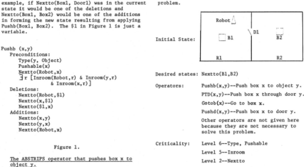
The operators are rules for transforming one state into another. For example, if the robot wanted to move Boxl to Box2 it would use the operator Pushb(Boxl, Box2) where Pushb is given in Figure 1. For this operator to be applicable, the pre conditions must be true of the current state, i.e., the preconditions give the domain of the operator. The current state is modified by de leting all of the formulae listed under deletions
and adding the formulae under additions. For
*
The reader will quickly note that this is illegal because the initial state is not in the domain of the operator. However, this subproblem is being solved at criticality level 6 which means that all predicates of level 5 or less are ignored. Nextto has been designated as level 2 and Inroom is level 5. Hence, at level 6, ABSTRIPS considers the Preconditions of Pushb(Bl, B2) (see Figure 1) to be Type(B2, Object) and Pushable(Bl) which is true in the initial state and consequently the opera tor is applied. Normally, several operators will be necessary to solve the problem but in this case one suffices.
The next subproblem, #2 in Figure 3, is to get from the initial state to a state in which the level 5 and higher predicates of the preconditions of Pushb(Bl, B2) are true. In Figure 3 we have only listed the predicates which are false in the initial state for purposes of exposition. (We are assuming that the variable r is assigned the value R2.) ABSTRIPS notes that PTD(Bl, Dl) is relevant to this subproblem and applies it which solves the subproblem. The level 2 predicates in the preconditions of PTD(Bl, Dl) are ignored be cause this subproblem is being solved at critica lity level 5.
Next, Pushb(Bl, B2) is applied to the result of this subproblem and this new state is transformed into a desired state. But is is already a desired state; i.e., applying (PTD(Bl, Dl), Pushb(Bl, B2) to the initial state results in a state which satisfies Nextto(Bl, B2). Hence, no subproblem
For the purposes of this report the details of the problem specification are not important. The important thing is that each problem has a state space, an initial state, a set of desired states, and a set of operators. Each operator is a par tial function from states into states. The domain of the operator is given by its preconditions. It should be noted that Pushb is really a partial function schema; it becomes a partial function after values are specified for x and y, i.e., Pushb(Boxl, Box2) is a partial function. The point is that ABSTRIPS is not dependent on the problem specification language but its underlying algebraic structure. Hence, ABSTRIPS could be applied to problems specified in the other langu ages such .as the one given in Ernst, et al (1974) in which states are represented by arrays.
3. Description of ABSTRIPS
ABSTRIPS assumes that each predicate in the pre conditions of operators has a criticality level assigned to it. (Actually Sacerdoti (1974) has a semi-automatic way of assigning criticality le vels.) The intuitive idea behind criticality levels is that high level predicates are more difficult to change than low level predicates.
A simple problem is given in Figure 2 and ABSTRIPS' solution is depicted in Figure 3. It starts off by trying to transform the initial state in Figure 2 into one in which Bl is next to B2. (This is subproblem 1 in Figure 3.) ABSTRIPS notes that the operator Pushb(Bl,B2) is relevant to this problem and applies it, which solves the is created in this situation. This completes the activity at criticality level 5.
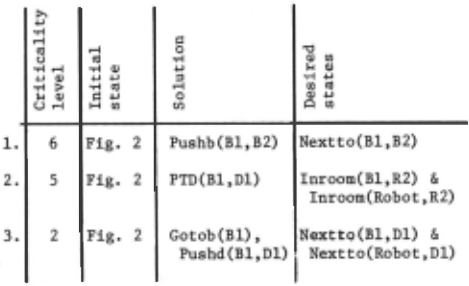
The next discrepancy shows up at level 2 because the preconditions of PTD at this level are not . satisfied. ABSTRIPS sets up subproblem 3 in Fi gure 3, and notes that Pushb(Bl, Dl) is relevant. However, this operator is not directly applicable because the level 2 predicates in its precondition are not satisfied. Gotob(Bl) rectifies this sit uation and hence (Gotob(Bl),Pushd(Bl, Dl)) is applied to the initial state which results in a states in the domain of PTD(Dl). Since this sub problem is solved, ABSTRIPS applies PTD(Dl) to s which yields a new state t and then attempts to transform t into the domain of Pushb(Bl, B2). All of the level 2 predicates in the preconditions of Pushb(Bl, B2) are considered because this subpro blem is being solved at criticality level 2. But , since tis already in the domain of Pushb(Bl, B2), this subproblem is trivially solved. Hence, Pushb(Bl, B2) is applied to t and ABSTRIPS at tempts to transform the result into the set of desired states. But the result is already a de sired state and thus this subproblem also has a trivial solution. Since criticality level 2 is the smallest level, the solutions of the subpro blems comprise a solution of the main problem.
To summarize, ABSTRIPS sets out to solve a pro blem at a given criticality level by essentially removing from the preconditions of all operators, predicates whose level are less than the given level. After finding a solution it goes to the next level down and adds the predicates at this level back to the preconditions of the appropri ate operators. This gives rise to subproblems that ABSTRIPS attempts to solve at the current criticality level, i.e., with lower level predi cates removed from operator preconditions. This process is repeated until the subproblems at the ~allest criticality level, wh~ch is 2 in the above example, are solved. Of course, there is search. involved at all levels because at any given level a problem may have several different solu tions some of which may generate unsolvable sub problems.
4. Planning
ABSTRIPS is quite similar to what Newell & Simon (1972) call planning. ABSTRIPS and planning dif fer in 2 major respects:
- Pl. Planning uses an entirely new problem solving space--both states and operators.
- P2. Planning uses only 1 level of abstraction while ABSTRIPS has one for each criticality level except the lowest which is the pro blem space itself.
Although planning does not presuppose criticality levels, they can be used to define the planning space. We will apply planning to the example of the previous section to contrast the two methods.
In the planning space of the problem in Figure 2 all of the level 2 predicates are removed. (In this example Nextto is the only level 2 predi cate.) Thus, a state in the planning space will be described exclusively by level 5 and level 6 predicates. All level 2 predicates are removed from operators to get the planning space opera tors. This includes the level 2 predicates in the addition and deletion lists as well as in the pre conditions of the operators. Of course, removing these predicates causes some operators to become identity maps, e.g. Pushb, in which case they are not used in the planning space. All level 2 pre dicates are removed from the formula that des cribes the desired states to get its analogue in the planning space. Hence, the planning desired states must be given by Inroom(Bl, R2) & Inroom (B2, R2). Removing the level 2 predicates from the description of the desired states in Figure 2, gives the null description which represents the set of all states.
The solution to the problem in Figure 2 in the . planning space is the single operator PTD(Bl, Dl). This generates 2 subproblems in the original pro blem space: transforming the initial state i .nto the domain of PTD (Bl, Dl), and transforming the result of applying PTD (Bl, Dl) to the solution of the first subproblem, into a desired state.
In general, planning is a two phase process: the first phase is to solve the problem in the plan ning space. The second phase is to elaborate the solution so that it works in the original problem space. This is done by inserting operators into the solution that was found in the planning space. The operators to be inserted are found by solving subproblems of transforming the appropriate states into the domains of the appropriate operators.
5. Formalization of A)!S_'IRIPS_ii~ _ _!'_l_!!!ffiing
Our formal model of ABSTRIPS is based on two as sumptions in addition to the above description.
- Al. The set of desired states is processed in the same way as the preconditions of operators.
- A2. When solving a subproblem at criticality level i, ABSTRIPS will reject any sub subproblems of criticality level greater than i.
By the first assumption we mean that at critica lity level i, ABSTRIPS will ignore all predicates less than level i in the description of the de sired states. This is what planning does. For example, the Nextto(Bl, B2) in the goal states of Figure 3 would be considered at level 2 but not at level 6. We are not suggesting that this is a good idea, but without it and A2 we could not characterize the solutions that ABSTRIPS can find. This will be discussed further in section 7.
The second assumption has to do with efficiency of search. Suppose ABSTRIPS is working at criti calitY level 2 on a Nextto predicate and an incorrect Inroom predicate is generated by at tempting to apply an operator. "Fixing" the Inroom predicate is a level 5 subproblem, but when it is considered at level 2 it is much more difficult because all of the level 2 and level 5 predicates are considered to be part of the operator precon ditions. Assumption 2 above specifies that all such subproblems are rejected as being too diffi cult.
At this point it is convenient to formalize the notion of the difficulty of a subproblem. A sub problem with initial state s and desired states T has difficulty i if there is a level i predicate in T which is not satisfied by s and all predi cates of higher criticality level in T are satis fied by s. We define Di(s, T) to be true if and only if the subproblem defined by s and T has difficulty i.
Only certain operators will be used to solve the subproblems of difficulty i; these operators will be denoted by Hi. To define Hi we first define the notion of relevance and irrelevance. The operator f is irrelevant to Di if for all s and T, Di(s, T) iff Di(f(s), T). That is, f is irrele vant to Di if it never changes the difficulty le vel of a subproblem of difficulty i. All opera tors f that are not irrelevant to Di are relevant to Di. We can now define Hi to be the set of operators which are relevant to Di but irrelevant to Dj for j > i.
The reason for these definitions is that all sub problems that ABSTRIPS attempts to solve at criti cality level i have difficulty i; i.e., Di(s, T) where s is the initial state and T is the desired states. In fact the reason for A1 and A2 is to make this statement true. ABSTRIPS actually violates A1 and hence considers some level 2 problems at level 6 as shown by the example in sec tion 3. It is not clear from the description in Sacerdoti (1974) whether or not ABSTRIPS adheres to A2. In any case our formal model assumes both Al and A2. The only operators that ABSTRIPS uses at criticality level i are in Hi. Of course, this is true because all subproblems at this level have difficulty i.
We formalize ABSTRIPS as a process which searches exhaustively, for well stratified solutions as defined below. Let (f 1 , ··· ,fk) be the solution of a subproblem whose initial state is s and whose desired states are given by T. That is, fk( .·· f 1 (s) · .· )ET and each intermediate state is in the domain of the appropriate operator. Below we will denote a subproblem by a pair (s,T) in which s is the current state and T is the set of desired states and Sf will denote the domain of the operator f. Define a non-empty subsequence ~i , fi ,
1 2 ... , fi ) t of the solution and an interger m such
that
- ii) fj t H for 1 ~ j ~ k & p > m· p ·
- iii) fj t H unless j = i where l~q~t. m q
This subsequence defines the following set of sub problems and a corresponding solution for each.
- If i 1 > 1, define (f 1 , ·.. ,fi _ 1 ) to be 1 the solution of (s, Sf ) · il
- For all j when 1 ~ j ~ t-1 and it 1 < ij+l define (fi +l' fi + 2 , ··· , j j f ) to be the solution of the ij+l-1 problem (fi ( ··· f 1 (s) ·.· ) , j ) .
- If it < k then define (fi +l' t ··· ,fk) to be the solution of f 1 (s) ... ),T).
Such a subsequence of a solution is called the stratification of the solution and the subproblems it defines are called its stratified subproblems.
This definition is conceptually much simpler than it appears to be, as shown by the following exam ple. Suppose that (f 3 , f 5 , f 6 , f 10 ) is the stratification of the solution (f 1 ,f 2 , ··· ,f 10 ) to the p·roblem (s,W). This stratification "groups"
,
the solution as (f 1 f 2 )f 3 (f 4 )f 5 f 6 (f 7 faf 9 )f 10 · Each of the parenthesized quantities are solutions corresponding to stratified subproblems. For example, (f 7 ,fa,f 9 ) is the corresponding solution to (f 6 ( ... f 1 (s) ··· ), Sf ). Note that there is 10 no subproblem between f 5 and f 6 . In addition, f 3 , f 5 , f 6 and f 10 are in some Hm and all the
other f's are in "smaller" H's.
and the corresponding solution of each of the stratified subproblems is well stratified. That is, each subproblem is of difficulty m. (Note that i-iii above only refer to the H's and not the D's.) The definition of well stratified is recursive since it requires all of its subpro blems to be well-stratified also. By the way the stratification subsequence is defined, m decreases with each level of recursion. Continuing with the above example, the solution is well stratified if all the difficulty of all top level subpro blems ism; e.g. , Dm(f 3 (f 2 (f 1 (s))),W). In addition all of the .stratified subproblems must be well stratified. For example, (fa) might be the stratif i cation of (f 7 ,fa,f 9 ) which groups it as (f 7 )fa(f 9 ). This indicates that f 7 is the cor responding solution of (f (···f 1 (s)···),Sf ). The - 6 a
difficulty of the subproblems in this stratifica
tion ism' where fa£ Hm' and m' < m; e.g.,
To summarize then our formal model of ABSTRIPS is an exhaustive search procedure for well stra tified solutions. Of course, ABSTRIPS uses a specific search strategy; i.e. first it looks for the stratification subsequence from "left to right" and then for subproblem solutions and back tracks in its own special way. We have not mo deled this search order. In addition, our formal model is only approximate since it has Al and A2 built into it.
Our formal model of planning is an exhaustive search procedure for well stratified solutions that have 2 levels. Again we do not model the order of search. Since planning uses Al, the only approximation used by our model is A2.
6. Totally-Ordered Solutions
GPS uses the strategy of working on difficult sub problems first, saving the easier subproblems for later. The difference ordering is used to speci fy the difficulty of a subproblem. This strategy is not complete in the sense that some problems
that have solutions cannot be solved using this strategy. Ernst (1969) has characterized the class of solutions that GPS can find as totally ordered solutions. Intuitively, a totally ordered solution is one which generates a sequence of states in which the difficulty is monotonically nonincreasing. In addition, all subproblem solutions are also totally ordered. The subpro blems of a solution are defined in terms of m 0 and i 0 · Given a solution (f 1 , ... ,fk) of a subproblem (s, T), let m 0 and i 0 be defined as follows:
- fj ' HP for p > m and 1 ~ j ~ k; 0
- 1 < i < k - 0
- iii) fi £ H m 0 0
- iv) fj ' H for l~j < i m 0 0
That is m 0 is the "highest level" of the operators in the solution and fi is the first of such 0 operators occuring in the solution. Let M(s, T) denote the difficulty of the subproblem. That is, M(s, T) = c if Dc(s, T) and not Dj(s, T) for j > c. Then (f 1 , ... ,fk) is a totally ordered solution to the subproblem (s, T) if
- M(fj( · ·· f 1 (s) · ·· ), T) ~ M(fj+l( ··· f 1 (s) ··· ),T) for 1 ~ j < k;
- ii) if i 0 > 1 then (f 1 , ... ,fi) is a totally 0 ordered solution to the subproblem (s,Sf ) · io
- iii) if k > i 0 then (fi + 1 , ··· ,fk) is a to o tally ordered solution to the sub.problem (fi ( ··· f 1 (s) ··· ) , T). 0
Totally-ordered is not only a characterization of the solutions that GPS can find but is also a characterization of the solutions that either ABSTRIPS or planning can find.
Theorem: Any well stratifies solution is totally ordered. The proof will not be given in this paper; the proof of this theorem, stated in a slightly different formalism, is given in Banerji and Ernst (1977). Although we have not proven the converse of the theorem we believe that it is true when "good" difference informations is used. If so, then the set of totally ordered solutions
is a characterization of the class of solutions that ABSTRIPS or planning or any other process that can find all .and only well stratified solutions can find.
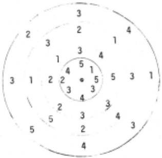
In Ernst (1969) a triangular table of connections was shown to be good difference information for GPS and it appears that this also specifies good parameters for ABSTRIPS and planning. Rather than giving a formal definition of a triangular table of connections we will give an example of it using the Fool's Disks problem. Figure 4 gives the initial state of the Fool's Disks problem, in which there are 4 concentric disks each containing eight numbers. These numbers line up so as to form 8 columns radiating from the center of the disks. A move consists of rotating one of the disks inde pendent of the others. The desired state is one in which each of the 8 radial columns sums to 12.
'-------- _ __/
Figure 4.
The initial state in the Fool's Disks problem.
| co ._ .... cs;; ._ 11"1 co ._ ""' ~ ._ ..... | c:: 0 ..... -:t ... ._ ::I ""' ..... 0 ..; ~ ._ M ..... | c:: 0 ..... ... c:: ::I 0 ..... ..... 0 ... ~ ::I ..... M 0 > N QJ ._ M ..... | |
|---|---|---|---|
| The vertical and horizontal diameters does not sum to 48. | 1 | 0 | 0 |
| Some diameter does not sum to 24. | 1 | 1 | 0 |
| Some radius does not sum to 12. | 1 | 1 | 1 |
A triangular table of connections for Fool's Disks.
A triangular table of connections for this pro blem is given in Figure 5. A 0 entry in the ta ble indicates that a difference is invariant over the operators. For example, the 0 in the upper right corner of Figure 5 indicates that turning a disk 1/2 revolution does not change the sum of the horizontal and vertical diameters. Note that Figure 3 has all O's above the main diagonal and no O's on it. The entries below the main dia gonal are unimportant. The difference ordering is just the row order; i.e., the top row heading is the most difficult difference while the bottom is the easiest.
GPS only uses the entries on the main diagonal to solve the problem. Hence, first 1/8, 3/8, 5/8 and 7/8 revolution of disks are used to remove the most difficult difference, i.e. used to get the horizontal and vertical diameters to sum to 48. Next, 1/4 and 3/4 revolutions are used to get each diameters to sum to 24. And finally the 180° moves are used to get a desired state. No tice that once a difference is removed it is never reintroduced because of the triangularity of the table in Figure 5.
7. Discussion
In the previous 2 sections we. made a number of highly technical definitions ending with a some what cryptic theorem, but what can be concluded from all of this? There are 3 major points, listed below; they are followed by a more general discussion.
Point 1. Given the "same" heuristic parameters planning, ABSTRIPS and GPS (or at least· our for mal models which approximate them) can all solve precisely the same class of problems, i.e. those that have totally ordered solutions. The rela tionship of parameters of the different methods is described below but note that the Di of Section 5 are just differences for GPS. This result is somewhat surprising because tne sear.ch space of GPS is quite different than that of planning or ABSTRIPS. For example, for all states s generated by GPS there is a path from the initial state to s. This is not true for planning or ABSTRIPS because many of the subpro blems may not be solvable. For any given problem probably one of the three methods is more effi cient than the others ·. but none is best for all problems.
Point 2. Selecting heuristic parameters can have a much more drastic effect on the search effi ciency than selecting one of the three methods, as shown by the Fool's Disks example above. The reason for this is that all of the methods are designed to search efficiently for totally ordered solutions; they will not even consider subproblems that give rise to unordered solutions. Totally-ordered is defined in terms of the para meters which are problem dependent, and hence the parameters determine ~hether the class of totally ordered solutions is the same as the class of all solutions or whether the former is much smaller than the latter. In fact, one can view the problem of selecting good parameters as the problem of making the class of totally ordered solutions as small as possible without eliminating all solutions to problems of interest.
Point 3. Any parameters which are good (in the sense of guiding search) for one method will have analogues which will be good for the other me thods. A triangular table of connections (see Section 6) is a property of good difference in formation for GPS. Another property of good dif ferences is given in Banerji and Ernst (1977). These properties, after suitable translation, are also properties of good parameters of planning and ABSTRIPS. Currently, we are implementing a program to discover difference information for GPS which satisfies these properties. Hence, this program effectively will discover good parameters for planning and ABSTRIPS also.
We feel that point 2 is the most important of the three points. Not much is known about the pro cess of selecting good parameters. Some initial work on this topic is outlined under point 3 but more research is needed on ·this topic.
To understand the above points, we need to know the relationship among the parameters of the 3 methods. The Di of Section 5 are just the differences of GPS. That is, subproblem (s, T) possesses differenced if Di(s, T) where d corresponds to Di. The subscripts on the D's give the difference ordering, e.g., the difference corresponding to D 2 in the example in Figure 2 is the easiest (smallest) difference because 2 is the smallest criticality level. The table of con nections indicate that the operators in Hi should be used to reduce Di. Note that in our formal models of both ABSTRIPS and GPS an operator f may be relevant to Di but not in Hi. This will happen when f E Hj for some j > i which indicates that f is relevant to the more difficult dif ference D1 and hence is used solely for the purpose oi reducing Dj. Including fin Hi would give rise to more search but not to more totally ordered solutions.
Planning, in many respects, looks like ABSTRIPS with 2 criticality levels. In fact our formal model of the previous section is really a hybrid of ABSTRIPS and planning; it has many levels of abstraction like ABSTRIPS, and like planning as sumes Al. The heuristic parameters of planning are basicly the difference information of GPS. Although planning requires a entire planning space as input, this information is really de rived from the difference orderin~. In fact one of the innovations in ABSTRIPS is its ability to automatically generate the various planning or abstracted spaces from the criticality levels of the predicates.
Our formal model of ABSTRIPS uses assumptions A1
and A2 (Section 5) which is a deviation from the real ABSTRIPS. Why might ABSTRIPS want to violate Al and/or A2? The answer lies in the fact that the class of totally-ordered solutions may be a little too restrictive because some solutions may not be totally-ordered. Violating Al and/or A2 allows ABSTRIPS to find solutions that are "almost but not quite" totally-ordered. We do not know how to measure the degree of unorderedness or what these violations due to the efficiency of search. To see how an unordered solution is generated note that ABSTRIPS' solution to the problem in Figure 2 is unordered because the difficulty of the original problem is level 2 whereas the difficulty of some of the subproblems is level 5. This un ordered solution is a result of violating Al. To have planning solve the problem in Figure 2 the desired states had to be more completely specified as described in Section 4 because planning adheres to Al.
What is the relationship of the properties of good differences in (Ernst, 1969) to the parameters of ABSTRIPS? As mentioned above the criticality levels of predicates basically specify the dif ferences and difference ordering. If the table of connections is generated as defined in Section 5 (i.e. use operators in Hi to reduce Di), then the properties of good differences are automatically satisfied except that some of the Hi may be empty. What this means is that if all solutions of a problem contain subproblems of difficulty i, then the problem has no totally-ordered solution. In other words the criticality level assigned to predicates is not good. A better approach is to ask what assignment of criticality levels results in no empty H's. This is very similar to the approach in Eavarone and Ernst (1970).
We feel that the biggest restriction in ABSTRIPS is its use of a very restrictive class of dif ferences, i.e., those defined by the predicates in the problem specification. Most of the good ideas in ABSTRIPS apply to a more general class of dif ferences; and we hope that the restriction is removed in the future. As an example of a dif ference not defined by a predicate in the problem specification, the logic task in Newell . and Simon (1972) uses the number of different proposition letters in an expression as a difference. Figure 5 also contains some more complex differences. We believe that ABSTRIPS can be extended to a wider class of differences such as these.
@inproceedings{ijcai1977p100,
  title     = {A Comparsion of Three Problem-Solving Methods},
  author    = {Banerji, Ranan B. and Ernst, George W.},
  booktitle = {Proceedings of the Fifth International Joint Conference on
               Artificial Intelligence, {IJCAI-77}},
  publisher = {International Joint Conferences on Artificial Intelligence},
  editor    = {Raj Reddy},
  pages     = {442--448},
  year      = {1977},
  note      = {Problem-solving and Search},
  url       = {https://ijcai.org/proceedings/1977/100},
}
TY - CPAPER TI - A Comparsion of Three Problem-Solving Methods AU - Banerji, Ranan B. AU - Ernst, George W. T2 - Proceedings of the Fifth International Joint Conference on Artificial Intelligence, IJCAI-77 PB - International Joint Conferences on Artificial Intelligence PY - 1977 SP - 442 EP - 448 UR - https://ijcai.org/proceedings/1977/100 ER -Copied
Machine-readable versions of this paper, for tools and AI agents:





