Some Properties of Small Networks of Randomly Connected Artificial Neurons

Introduction

Much of the work on brain models in the late 1950's and early 1960's comprised the construc­ tion, either in hardwar~, or more commonly by simulation on a digital computer, of networks of artificial neurons (hereafter the term 'neuron' will refer to ·artificial neurons, where necessary brain cells will be referred as 'natural neurons'). Historically the idea networks of neurons performing brain like functio~s stems from the work of McCulloch and Pitts.

Si~ilar work was presented and expanded by Kleene , who showed that it is possible to represent any definite event (i.e. an event comprising a definite set of input sequences but not an event whose input sequences extend indefinitely into the past) in a finite automaton which could be constructed from McCulloch-Pitta neurons. Unfortunately this work is of little practical help to model builders, it points out some of the possibilities and limitations of the excercise without giving any firm guidelines as to the construction of such models.

The process of neuron modelling adopted by various workers has tended to follow a fairly fixed pattern, starting with a description of some of the generally assumed properties of natural neurons, and the interconnections between them, giving a framework for the construction of a network of neurons. These networks have then received discrete or continuous input stimulation and some record made of the resultant pattern of activity. There may or may not be any modifi­ cation (adaption) of the network parameters to attempt to demonstrate learning by the network.

Generally assumed properties of neurons

Most model neurons incorporate all or many of the following features (see fig 1). The inputs to· a neuron may be either excitatory, e., (positive) or inhibitory, i., (negative). Eacfi input connection has a certdin weight ascribed to it, if an impulse is received along a ' particular fibre an amount of excitation (positive or negative) proportional to the weight of the connection is given to the neuron. The neuron is a threshold device; it has an 'all or none' mode of operation and will only produce an out- R. L. Beurle, Department of Electrical and Electronic Engineering, The University, Nottingham, England.

put (fire) if its excitation exceeds a certain predetermined (threshold) value,

Thus the neuron will fire if

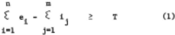
where T is the threshold and e is proportional to the weight of the ith. excitatory connection if an input pulse has just been received along .ith. fibre, and zero otherwise (sim. for ij).

The neuron does not transmit an output pulse as soon as the excitation exceeds the threshold value, there is a short delay - corresponding to the synaptic delay in natural neurons - before on output pulse is transmitted. Although in natural systems a neuron may apparently fire at any time, in simulation experiments it is only possible. to deal with discrete time intervals, thus the synaptic delay time, t, is usually taken as the unit of time. Therefore ifat time t - 1 a neuron receives an amount of excitation greater than its threshold value it will transmit an output pulse at time t = 0 to all neurons connected to its axon branches, this output becomes an input to these neurons at time t : o, unless some speed of travel constraint is applied to the connections. Normally all cells with which an axon system connects receive inputs in the same time interval irrespective of their distance from the originating cell.

If a neuron does not fire in a particular time step after receiving some excitation then, in many models, its excitation does not immediately drop to zero but falls exponentially towards zero with a time constant usually of the order of 0.1 to 2 time intervals. Hence a neuron may fire after repeated bursts of stimulation, none of which by itself is sufficient to fire the cell; this is observed to occur in natural neurons.

Also, in order to comply with neuro­ physiological data, immediately after a cell has fired its threshold becomes infinite this state (the absolutely refractory period) ~~ually lasts 1 to 3 time intervals. The threshold then decays towards its quiescent value, again it is convenient to assume an exponential decay with a typical time constant of 0.2 to 3 time steps. These points are illustrated in fig. 2.

The connections from cell to cell are unidirectional and independent (pulses may only travel as output from one cell via its axon branches to provide inputs to other cells, but there is no reason why if an axon branch of cell a is connected to cell b that an axon branch of cell b should not be connected to cell a). The connections are distributed according to some rule, normally a function of the radial distance between cells.

Some feedback mechanism may be be applied to the network in an attempt to cause it to produce particular forms of output in response to particular inputs. Mechanisms of the form - if the required output is not obtained reduce the weights of all connections which contributed to the firing of cells and increase the weights of all those which fed pulses to cells which di1 not fire - have been used with some success. If inhibitory as well as excitatory connections have been used then some originally positive (excitatory) connections may become negative (inhibitory) by the use of such mechanisms. This has been the case in several models, but it is believed that this is not physically possible in natural systems, where a synapse appears to be 9 always either excitatory or inhibitory. Uttley has suggested that this difficulty may be overcome by postulating that there are always two pathways connecting any two neurons, a direct excitatory pathway, and an indirect (via an intermediate neuron) inhibitory pathway.

To summarise we have the following parameters for each cell.

• T Threshold
• Excitatory connections Inhibitory connections Denoting cell of origin and

weight

• Excitatory connectivity function r is the radial dist­
• Inhibitory connectivity function ance between cells.

Synaptic delay (basic unit of time)

Absolutely refractory period

Refractory period time constant

Excitation decay time constant

Excitatory weight modification function

Inhibitory weight modification function

7 x 7 Networks

Several networks were simulated and their performance examined on the Atlas computers at Manchester and Harwell. The type of neuron programmed incorporated most of the features described in section 1, the networks being con­ ceived as plane square matrices normally having a side length of 7 cells.

The cells were connected randomly with a given, variable exponential probability distribu­ tion of connections (see fig 3). The number of connections per cell might vary from about 5 to 25 depending on the parameters fed into the program data. For each cell, for each possible connection either to every other cell or .to all cells within a certain radial distance, a random number in the range 0 - 1 was generated (using a pseudo-random number generator sub-routine), if the probability of connection was greater than the random number produced then a connection was established between the two cells. Thus the constant 'A' (fig. 3) effectively controlled the number of connections per cell (for a given 'a') and the constant 'a' the distance decay of probability of connection. _The program was arranged such that a cell could not be connected to itself.

In many of these models the connection pattern for each cell was calculated and stored separately, as far as the author is aware in all other simulation studies a repetitive from of connection has been used. Some later networks were constructed with a repetitive connection pattern and are compared with the previous models in section 7. In the 7 x 7 models only excitatory connections of fixed weight were used. A quies­ cent threshold level, To, of 200 was chosen, and a value of 1000 to represent the initial point, Tm, for the decay of the refractory period, Two forma of refractory period were used:-

1. lat. time step after firing, cell absolutely refractory

2n1· time step after firing, threshold · /2 To

3rd. time step after firing, threshold '"To

1. lat. time step after firing, cell absolutely refractory

2nd. to nth. time steps governed by the expression

where El is a constant less than unity, g is the nuhlber of time steps since the cell last fired

(n + l)th. time step after firing, threshold · To

For type (b) temporal summation of excit­ ation was effected by using the relation

where Et is the excitation level at time t, and E2 1s a constant less than unity.

Values of El used were 0.4, 0.7

Values of E2 used were 0.5, 0

There was no temporal summation of stimuli for type (a) networks.

The advantages of using a pseudo-random number generator were that the same sequence of statistically random numbers could be produced repeatedly merely by starting the generation sequence with the same 'priming' number, this enabled the same network to be set up on the computer on different occasions without having to read in the connection details as data; and also networks with the same connection parameters

(density of connections, and probability of connection distribution) could be set up and compared by simply regenerating the network using a different priming number.

For each time step a cell which has just fired is denoted by the symbol 1, and a cell which has not fired by the symbol 0.

Description of results - 1st series

7 x 7 networks of neurons were set up on the computer as described above, in this first series of experiments the inter neuron connections were calculated and stored separately for each cell in the network. The network was initially stim­ ulated by exciting three or four of the nine central cells with one of the patterns shown in fig. 4.

The activity was allowed to continue for a number of time steps, usually 20 or 40, the activity was then stopped, all cells returned to their quiescent state with zero excitation, and a new pattern of activity initiated by stim­ ulating the network with a different 'input pattern. Provision was made to output the activ­ ity pattern in the network at each time step, or for the final few time steps.

The type of activity which occurred in the networks . fell into one of five categories. Examples of which are shown in figs. 5 - 9.

1. Attenuation. The connectivity of the network is not sufficiently 'strong' and the activity dies out in a few time steps. (fig. 5)
2. Unstable. The activity does not atten­ uate, but there is no discernible continuing cyclic pattern; at least in the short term. (fig. 6)
3. Virtually stable (a). With the number of time steps recorded the output has not satisfied one of the conditions 4 or 5 (see below), but it appears probable that it .will lock in to one of these modes during the next few time steps. (fig. 7)
4. Virtually stable (b). The output pattern at time t is not identical with that at time t + 2, but is identical with that at some time t + n, where n is an integer greater than 2 (fig. 8)
5. Stable. The network produces an oscillatory output such that all cells which do not fire at time step t, fire at time step t + 1. All cells which fired at time step t are of course absolutely refractory at t + 1. The t th. pattern is therefore the inverse of the pattern of the previous time step, and identical with the (t + 2) th. pattern. (fig. 9)

From an examination of the outputl!l typified in figs. 5 - 9 several features emerge.

The distinction between modes 2 - 4 is some­ what arbitary and more one of degree than a pre­ cise division . Those networks classified as type 3 normally only lack stability in a few (say iess than 6) 'outer square' cells. In type 2 networks there is a more random variation, frequently some cells change allegiance; i.e. if they were initially ON during an even time step they may, at a latter stage, be ON during an odd time step. In such unstable networks no two identical out­ puts have been noted over periods of 40 time steps (the exponential refractory period lasted 5 time steps). It is difficult to imagine that one of these networks if allowed to maintain activity for a sufficiently long time would not fall into a cycle, even if this were of many hundreds of time steps duration. An interesting feature of this type of network is the tendancy for underlying patterns of activity (similar to type 4) to last for a few time steps, slowly disintegrating to form a new basic pattern which .in turn builds up and then disintegrates - though a few cells may be common to all such transitory patterns.

The difference between modes 5 and ~ is presumed to be a lack of specific connections to a particular cell or cells, such that they only fire every 4th. or 6th. time step rather than every 2nd. step. It is also possible for a cell to fire every 3rd. time step giving a mode 4 output with a cycle time of 6 time steps.

The lock in time before a stable output was produced was affected by the type of input pattern used to stimulate the network. Networks stimulated with patterns i and ii tended generally to stabilize more rapidly than iii and iv type inputs due to their having a greater probability of two or more active connections to the same cell during the first time step. For example in patterns i and ii there are six cells which are only one unit distance from two stimulated cells, in iii and iv there are only four such cells. In v there are nine such cells, but insufficient runs were made to satisfactorily compare the tendency of this input to stabilize quickly compared with types i - iv.

The lock in time is also dependent on the constant 'A' being shorter for large values of A. For sufficiently large A the network will stab­ ilize instantly to repeat the input pattern unchanged in alternate time steps (fig. 10). This 'over connected' network gives rise to an inter­ esting and possibly useful mode of activity which it is convenient to designate as mode 6 - the saturated stable mode.

To summarise, dependent on the network para­ meters the flow of activity in the network will give rise to one of six possible modes. These are:-

1. Attenuation
2. Unstable
3. Virtually stable (b)
4. Stable
5. Virtually stable (a) 6.
6. Saturated stable

Comments on results - 1st series

The results of this first series of experiments raised several points on the behav­ iour of these and more complicated networks. Many of these were in the form of a more accurate assessment of the variation in output with the various network parameters, e.g.

1. What is the effect of the threshold/connect­ ivity strength ratio on the stability of the network - perhaps expressed in terms of the lock in time and the period of the cyclic activity.
2. A quantitative analysis of the effects of 1 A 1 , 1 a 1 , the length of the absolutely refractory period, the refractory period decay constant and the excitation decay constant on the network.
3. The effect of the variation of input pattern size and shape on the tendancy to produce different modes of operation.

The most interesting form of activity which the networks produced was their ability to give a stabilized output of short cycle length. As far as the author is aware this property has not been previously demonstrated. Presumably because of the shortage of computing storage and time other workers have tended only to output the frequency of firing of cells, or monitor the gross activity of the network. Hence they may not have realised that the nature of the activity - even when they observed stability - was such a fine measure of the input pattern.

The stabilized pattern is always character­ istic of the particular input pattern initiating the activity (fig. 11), though it is possible that two different input patterns could give rise to the same output activity, but this has not been observed to occur. With a lightly connected network the output pattern for a given input pattern varies with the connectivity, i.e. it is dependent on the particular random number generator (b) used (fig. 12). However, when there are sufficient intercell connections a pattern may be set up which duplicates the original input pattern in alternate time steps independent of the particular connectivity generator.

This latter form of activity is interesting for it shows that a very simple network, having neurons with only excitatory connections to other cells, can exhibit a useful memory function. The requirement is that there should be a large number of such connections but these may be made at random, the activity pattern being independent of the actual connectivity pattern. Once stim­ ulated the network is unaffected by additional excitatory inputs; the pattern once established cannot be altered except by inhibiting some of the cells from firing in a particular time step. This is so because every cell which is not absolutely refractory fires as soon as it has emerged from its absolutely refractory period. Thus we have a mechanism which can be used to store an input pattern indefinitely and which is unaffected by subsequent excitatory inputs to the network. The network may be returned to its quiescent state by applying blanket inhibition over the whole network.

These networks therefore possess some possibly useful properties, in order to further evaluate these properties a second series of networks was simulated.

Second Simulation

A major drawback to the method used to construct the original networks - calculating the connectivity pattern for each cell - was the large amount of .computer storage which had to be allocated for this purpose, also causing a consequent increase in computing time. This was so severe that practically it was impossible to run the simulation for networks of much more than 100 cells, and potentially restrictive on the number of runs which might be made to evaluate the properties of 7 x 7 or similar networks. Accordingly a modified program was written in which a more regular connectivity pattern could be adopted, but hopefully have no significant effect on the performance of the network compared with the original model. A program of this type was essential if larger networks with inhibitory and excitatory connections were to be simulated.

Comments on 7 x 7 networks - 2nd. series

In order to evalute the performance of 7 x 7 networks various network parameters were varied in turn, holding all other parameters constant. There being several variables it is difficult to adequately portray the performance in graphical form. Nevertheless figs. 13 & 14 give an impression of the behaviour of the networks.

It will be recalled that the connectivity of the network is governed by the expression

where A, a are constants, and r is the radial distance between cells, and that a connection is made if

where x is a randomly generated number on the range 0 - 1.

The form of activity sustained in the net­ work as A and a are varied is shown in fig. 13. For large A and a saturated stable activity (mode 6) occurs, as the value of these constants is reduced -this activity gives way to the stable mode (5), initially with immediate lock in to the mode, and only one or two cells in addition to the originally stimulated cells firing in 'odd' time steps. As A and a are further reduced the following progression of activity takes place: the lock in time to mode 5 gradually increases, and more cells fire in odd time steps, when the lock in time is about five or six time steps and about half the cells are ON in each time step, the activity changes to mode 4 with immediate lock in time. At this stage the mode 4 activity will generally have a cycle time of six time steps, or occasionally four time steps. Then the cycle and lock in times gradually increase until no purely cyclic activity is noted over a period of 20 or so time steps, mode 3. Though in these cases the central 25 cells usually cycle with a short cycle time, and instability is confined to the outer ring of cells. Where longer simulations have been made these networks tend to have very long lock in and cycle times, the latter were usually a multiple of 6, which was the total length of the refractory period used. A very narrow band of unstable (mode 2) activity occurs between mode 3 and mode 1 (attenuation). In this region the pattern in the central core of cells changes and the instability is no longer confined to the outer ring of cells. Though s'ome repeated patterns have occasionally been noted in simu­ lations of 40 or more time steps no tendancy to cyclic activity has been noted. The activity in this mode is either a very extreme case of mode 3 with exceedingly long, probably greater than 100 time steps cycle time (c.f. reference 8), or alternatively activity which will ultimately attenuate; a case has been observed where the activity attenuated after some 20 time steps. Near the virtually stable region activity attenuates (mode 1), initially activity lasts for a short period, as A and a are reduced this period decreases until the activity dies out immediately after stimulation. There is a gradual drift of the mode division curves towards the origin as the number of cells initially stim­ ulated rises to half the total number of cells, but this effect is very slight for small numbers of cells initially stimulated, the curves for 3 and 7 cells being virtually identical. All the mode division curves will become asymptotic to the A and a axes, since for both A = 0 and a = 0 there can be no connections to other cells, but for a value of one variable near zero, and a very large value for the other sustained activity is possible.

Figs. 14 a d show the effects of varying both the quiescent threshold and the maximum threshold following the absolutely refractory period for different values of a, all the graphs being drawn for a value of A = 1. The threshold decay was controlled by equation 2.

As the quiescent threshold rises it becomes more and more difficult to initiate sustained activity, when the connectivity is strong enough for sustained activity to occur there is a corresponding increasing tendancy for it to be stable, and the region (modes 2, 3 and 4) of virtually stable and unstable activity becomes very narrow (fig. 14d). For larger values of A

the mode division boundaries will move upwards and to the left. In the same manner as fig. 13, there is a gradual change from one form of activity to another, but the mode division , boundaries are surprisingly clear, very rarely is a network found which does not respond in a manner which could be predicted from the graphs. In these rare cases where the activity has not been in the predicted group it has, except in one case, been of the form of the nearest adjacent region.

Different random number generators, b's, have little effect on the form of figs. 13 and 14, occasionally a network, whose parameters place it very near a mode division boundary, will change from one mode to the other for different gen­ erators, but normally the activity may be acc­ urately predicted. Thus the value of 'b' used does not seriously affect the prediction, it merely adds the additional constraint that for certain critical values of the network parameters the activity mode will be dependent on the actual network connections.

This second series of experiments has shown that the specification of the parameters A, a, T , and T is sufficient to predict the behaviour o~ the ne~ork, and that the particular random number generator will usually only affect the form of the output pattern, as in fig. 12.

Modified simulation program

The method of generating the connectivity pattern used in the experiments so far discussed is satisfying in that a unique set of connections is generated for each cell, within the same statistical constraints as the connections to other cells. However, this method is wasteful in terms of computer storage, and to a lesser extent time. Therefore in the modified program instead of generating the connection pattern separately for each cell four possible connection patterns were generated; being the same as four arbitrary patterns which might have been generated by the original programme. Each cell in the network was assigned one of these connection patterns at random, the connectivity thus being a compromise between the original connection method and a purely repetitive method.

A series of 7 x 7 networks was set up using this connection technique and the performance of the networks compared with the original net­ works as depicted in fig. 13. It was found that the performance was in general very similar, but that the results were not quite so consistent. With the original networks, given the parameters A, a, a network's behaviour may be accurately predicted. In the modified system there was a far greater probability, perhaps 0.25 that the form of the activity would not lie within the regional boundaries of fig. 13, compared with about an 0.05 probability for the original net­ works. This is not altogether a surprising result, since if any one of the four connectivity patterns gives a 'poor' distribution of connectiona this will affect about a quarter of the cells, whereas the odd poor distribution in the original program will have little effect. How­ ever, within this restriction the second program gives a satisfactory simulation method.

Possible extensions of 7 x 7 networks

The stability of neuron has been discussed by several authors 1, 2, 6, 7, with the conclu­ sion that either some fairly complicated feed­ back mechanism monitoring the level of activity in the network and holding it within certain limits is necessary to prevent saturation. Or, as was then not such a popular idea with neuro­ physiologists but is now generally accepted as being the case, inhibitory as well as excitatory connections are necessary. To some extent in a small network, such as the 7 x 7 networks, these mechanisms are unnecessary since the absolutely refractory period ensures that all the cells can never fire at the same time - unless they were originally all stimulated together, in which case the activity will extinguish itself immediately if the excitation of a cell falls to zero once it has fired. Alternatively, if the excitation is merely reduced by its normal decrement, the network may exhibit saturated stable oscillation with all cells on in one time step, and none in the following step . Else, if the connectivity were strong enough to allow activity to continue but not to allow the saturated mode to occur the network would settle in one of the modes 3 - 5.

These forms of activity only suggest possibly useful applications in a small network, in a large homogeneous network (one with the same connectivity function throughout the network) if the connectivity is sufficiently strong such that activity does not attenuate then the activity will slowly spread throughout the network and will probably set up modes of activity very similar to those in 7 x 7 networks, but ~ith much greater lock in times. Fig. 15 shows how the activity has spread through a 50 x 50 network 15 time steps after being stimulated with a three cell input pattern.

It is useful to ask at this point whether the form of stabilized output which is easily demon­ strated in a small 7 x 7 network can be found to exist locally in much larger networks, without the activity spreading through the whole network as in fig. 15. One possibility is that in addition to the short range excitatory connections so far postulated we add a number of long range inhibitory connections, thus each local area when stimulated is surrounded by a barrier of inhibited cells (fig. 16). In principle we may now construct a model with this form of connec­ tivity, stimulate a small area of the network and observe if stable local activity occurs. If this is so we may further note the number of such stable systems which can be operated in a given size of network. It is not being proposed that distinct excitatory and inhibitory areas are set up in the network, but that the network is homogeneous with short range excitatory connec-

Networks with inhibitory and excitatory connect ions

Using the modified program a small number of 28 x 28 networks with inhibitory as well as excitatory connections were simulated. The net­ works had a homogeneous connection pattern, the excitatory connections being precisely as described above. Only one pattern of inhibitory connections was used, being common to all cells, again this was of the usual form governed by equation 4, except that no inhibitory connections were made to cells less than five cells distant. The connectivity constants (now denoted by Ai, ai, and Ae' ae' for inhibitory and excitatory · connections) could be varied independently.

From the results obtained it seems likely that the form of activity suggested earlier - a stable excited area surrounded by an inhibitory barrier - may be produced. Fig. 17 shows the activity in such a network after the 9th. and lOth. time steps. The activity in the lOth. step is identical with that of the 6th., and differs in only four cells from that of the 8th. The network is apparently exhibiting mode 4 activity, but this activity is limited to one area of the network. The tendancy for the activity to con­ centrate in a horizontal band appears to be a function of the particular connectivity generator used. With longer range excitatory connections, and weaker inhibition, pockets of activity may be stimulated in other parts of the network beyond the inhibitory barrier. In these cases activity will presumably spread throughout the network as in fig. 15, but at a much slower rate. No attempt has been made to evaluate the properties of the network in the manner of the 7 x 7 networks, or to initiate activity in two independent areas.