
Belief-Contraction-Driven Active Inverse Source Localization and Characterization
Proceedings of the Thirty-Fifth International Joint Conference on Artificial Intelligence. AI4Tech: AI Enabling Technologies. Pages 6528-6535.
https://doi.org/10.24963/ijcai.2026/726
Keywords
- Advanced AI4Tech: Deep AI4Tech
- Advanced AI4Tech: AI4Tech foundations
- Advanced AI4Tech: Data-driven AI4Tech
Abstract
Active inverse source localization and characterization (ISLC) in dynamic fields requires sequential decision making under partial observability, where a mobile sensor must infer latent source parameters from sparse, noisy readings. We introduce a belief-contraction-driven approach that unifies inference, stopping, and control. An attention-augmented particle filter stabilizes Bayesian belief updates through ESS-based resampling, feature-aware sparse attention smoothing, and Metropolis–Hastings rejuvenation that preserves the filtering posterior. Belief contraction (posterior dispersion) defines both a termination rule and a goal-aligned intrinsic reward, enabling reinforcement learning without distance-to-source shaping. Across seven field modalities, spatial out-of-distribution tests, and nonstationary source shifts, our agent (ATT-PFRL) achieves higher completion, faster convergence, and more accurate localization than planning and RL+Bayes baselines under similar computation. Fixed-trajectory studies also show improved ESS and lower RMSE, isolating the benefit of the inference layer.
- [Balkovsky and Shraiman, 2002] Eugene Balkovsky and Boris I Shraiman. Olfactory search at high reynolds number. Proceedings of the national academy of sciences, 99(20):12589-12593, 2002.
- [Chen et al., 2021] Wen-Hua Chen, Callum Rhodes, and Cunjia Liu. Dual control for exploitation and exploration (dcee) in autonomous search. Automatica, 133:109851, 2021.
- [Farrell et al., 2005] Jay A Farrell, Shuo Pang, and Wei Li. Chemical plume tracing via an autonomous under- water vehicle. IEEE Journal of Oceanic Engineering, 30(2):428-442, 2005.
- [Filippi et al., 2010] Sarah Filippi, Olivier Cappé, and Aurélien Garivier. Optimism in reinforcement learning and kullback-leibler divergence. In 2010 48th Annual Allerton Conference on Communication, Control, and Computing (Allerton), pages 115-122. IEEE, 2010.
- [Haarnoja et al., 2018] Tuomas Haarnoja, Aurick Zhou, Pieter Abbeel, and Sergey Levine. Soft actor-critic: Off-policy maximum entropy deep reinforcement learning with a stochastic actor. In International conference on ma- chine learning, pages 1861-1870. PMLR, 2018.
- [Holley, 1969] Edward R Holley. Unified view of diffu- sion and dispersion. Journal of the Hydraulics division, 95(2):621-632, 1969.
- [Hu et al., 2019] Hangkai Hu, Shiji Song, and CL Phillip Chen. Plume tracing via model-free reinforcement learn- ing method. IEEE transactions on neural networks and learning systems, 30(8):2515-2527, 2019.
- [Hu et al., 2025] Kun Hu, Muning Wen, Xihuai Wang, Shao Zhang, Yiwei Shi, Minne Li, Minglong Li, and Ying Wen. Pmat: Optimizing action generation order in multi-agent reinforcement learning. arXiv preprint arXiv:2502.16496, 2025.
- [Hutchinson et al., 2018a] Michael Hutchinson, Cunjia Liu, and Wen-Hua Chen. Information-based search for an at- mospheric release using a mobile robot: Algorithm and experiments. IEEE Transactions on Control Systems Tech- nology, 27(6):2388-2402, 2018.
- [Hutchinson et al., 2018b] Michael Hutchinson, Hyondong Oh, and Wen-Hua Chen. Entrotaxis as a strategy for au- tonomous search and source reconstruction in turbulent conditions. Information Fusion, 42:179-189, 2018.
- [Li et al., 2022] Zhongguo Li, Wen-Hua Chen, and Jun Yang. Concurrent active learning in autonomous air- borne source search: Dual control for exploration and exploitation. IEEE Transactions on Automatic Control, 68(5):3123-3130, 2022.
- [Lillicrap, 2015] TP Lillicrap. Continuous control with deep reinforcement learning. arXiv preprint arXiv:1509.02971, 2015.
- [Lochmatter et al., 2008] Thomas Lochmatter, Xavier Raemy, Loïc Matthey, Saurabh Indra, and Alcherio Marti- noli. A comparison of casting and spiraling algorithms for odor source localization in laminar flow. In 2008 IEEE International Conference on Robotics and Automation, pages 1138-1143. IEEE, 2008.
- [Mnih et al., 2015] Volodymyr Mnih, Koray Kavukcuoglu, David Silver, Andrei A Rusu, Joel Veness, Marc G Belle- mare, Alex Graves, Martin Riedmiller, Andreas K Fidje- land, Georg Ostrovski, et al. Human-level control through deep reinforcement learning. nature, 518(7540):529-533, 2015.
- [Park et al., 2022] Minkyu Park, Pawel Ladosz, and Hyon- dong Oh. Source term estimation using deep reinforce- ment learning with gaussian mixture model feature extrac- tion for mobile sensors. IEEE Robotics and Automation Letters, 7(3):8323-8330, 2022.
- [Schulman et al., 2017] John Schulman, Filip Wolski, Pra- fulla Dhariwal, Alec Radford, and Oleg Klimov. Prox- imal policy optimization algorithms. arXiv preprint arXiv:1707.06347, 2017.
- [Shi et al., 2024] Yiwei Shi, Kevin McAreavey, Cunjia Liu, and Weiru Liu. Reinforcement learning for source location estimation: A multi-step approach. In 2024 IEEE Interna- tional Conference on Industrial Technology (ICIT), pages 1-8. IEEE, 2024.
- [Shi et al., 2025] Yiwei Shi, Muning Wen, Qi Zhang, Weinan Zhang, Cunjia Liu, and Weiru Liu. Autonomous goal detection and cessation in reinforcement learning: A case study on source term estimation. In Proceedings of the AAAI Conference on Artificial Intelligence, volume 39, pages 738-745, 2025.
- [Steiner and Bushe, 2001] H Steiner and WK Bushe. Large eddy simulation of a turbulent reacting jet with conditional source-term estimation. Physics of Fluids, 13(3):754-769, 2001.
- [Vergassola et al., 2007] Massimo Vergassola, Emmanuel Villermaux, and Boris I Shraiman. 'infotaxis' as a strategy for searching without gradients. Nature, 445(7126):406- 409, 2007.
- [Zhao et al., 2022] Yong Zhao, Bin Chen, XiangHan Wang, Zhengqiu Zhu, Yiduo Wang, Guangquan Cheng, Rui Wang, Rongxiao Wang, Ming He, and Yu Liu. A deep reinforcement learning based searching method for source localization. Information Sciences, 588:67-81, 2022.
References were extracted automatically from the PDF and may contain errors.
Full text extracted automatically from the PDF; figures, tables and equations may differ. The PDF is the version of record.
1 Introduction
Accurately and rapidly localizing unknown sources in spatially distributed fields, such as gas leaks, pollutant releases, or electromagnetic anomalies,is a critical capability for industrial safety, environmental monitoring, and emergency response. These tasks are commonly formulated as Inverse Source Localization and Characterization (ISLC), where the objective is to infer latent source and environmental parameters (e.g., source position, intensity, and transport conditions) from sparse, noisy, and localized measurements collected by a mobile agent [Steiner and Bushe, 2001]. Active ISLC is inherently a partially observable sequential decision-making problem. Observations are local and often weakly informative, while the latent parameters remain unobserved; thus, effective behavior must be conditioned on a belief over those parameters rather than on raw measurements alone. This setting creates three practical challenges. First, intermediate feedback is sparse and implicit: the environment typically does not provide dense rewards that indicate progress toward successful localization, making reinforcement learning (RL) unstable or heavily dependent on hand-crafted shaping. Second, maintaining a reliable posterior under sparse/noisy sensing is non-trivial: standard particle filters can suffer from weight degeneracy and resamplinginduced particle impoverishment, leading to overconfident yet unreliable beliefs. Third, real deployments demand robustness across varying field modalities and distribution shifts (e.g., changed wind or spatial regimes), where reactive heuristics or narrowly trained policies may fail to generalize.
∗Corresponding author.
Prior work approaches ISLC through Bayesian planning and information-theoretic search [Vergassola et al., 2007; Hutchinson et al., 2018a], bio-inspired plume tracing and casting strategies, or deep RL methods for adaptive exploration [Zhao et al., 2022; Hu et al., 2019; Park et al., 2022]. However, existing solutions often face a trade-off between (i) principled inference and (ii) goal-aligned control. Information-theoretic planning can be computationally demanding and sensitive under partial observability, while RL approaches frequently rely on reward shaping that may be misaligned with the true objective (pinpointing the source) and can generalize poorly across conditions.
In this paper, we propose a belief-contraction-driven framework that couples Bayesian belief maintenance with belief-conditioned decision making for active ISLC. Our key idea is to treat posterior contraction-the reduction of uncertainty in the inferred belief-as the common objective that links inference, termination, and learning. Concretely, we (i) maintain a particle-based posterior over latent parameters and (ii) use a contraction criterion (based on posterior dispersion) as a task-completion signal and as a sparse intrinsic reward for learning. This converts implicit "mission completion" into an explicit, goal-aligned learning signal, avoiding distance-to-source shaping and directly reflecting whether the agent has localized the source with sufficient confidence.
To make belief contraction meaningful and robust under sparse/noisy sensing, we introduce an attention-augmented particle inference layer that mitigates degeneracy while controlling computational overhead. Starting from sequential importance sampling, we stabilize belief updates via (1) ESStriggered resampling when weight collapse is detected, (2) feature-aware sparse attention smoothing that redistributes weight mass among feature-similar hypotheses as a controlled perturbation on the simplex, and (3) MCMC rejuvenation with Metropolis-Hastings correction to restore diversity while preserving posterior invariance. The resulting belief state (posterior moments and uncertainty summaries) serves as the input to an execution policy. In this work, we instantiate the executor as an RL agent,ATT-PFRL,that learns exploration strategies conditioned on the belief, optimizing the sparse contraction-based intrinsic reward until the termination criterion is met. We validate the proposed framework in a suite of ISLC environments spanning diverse field modalities and challenging shifts. We further evaluate out-of-distribution spatial shifts and nonstationary source changes, highlighting robustness to distribution mismatch and dynamic regimes. To isolate inference improvements from policy-induced data collection, we additionally conduct fixed-trajectory evaluations that compare inference variants under identical observation sequences, and we perform dedicated analyses of cessation threshold sensitivity and intrinsic reward design, verifying that the contraction signal is calibrated against ground-truth localization quality.
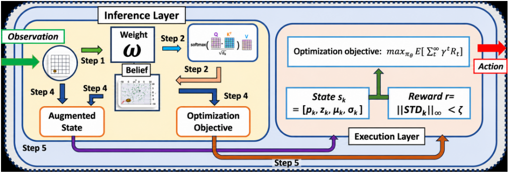
Our main contributions are: 1.) A unified framework that aligns inference, termination, and learning by using posterior contraction as both a stopping criterion and a sparse intrinsic reward for belief-conditioned control. 2.) An efficient degeneracy-mitigation pipeline combining ESS-triggered resampling, feature-aware sparse attention smoothing, and MH-corrected rejuvenation to stabilize belief updates under sparse/noisy observations while preserving posterior correctness. 3.) Extensive experiments across diverse field types, out-of-distribution regimes, and nonstationary shifts, including inference decoupling and reward/cessation validations that directly support the proposed design choices.
2 RelatedWork
Traditional planning-based methods for ISLC typically fall into two categories: Information-Theoretic Approaches and Bio-Inspired Methods. The former strategies aim to reduce uncertainty about the source location, with Infotaxis [Vergassola et al., 2007] minimizing posterior variance, Entrotaxis [Hutchinson et al., 2018b] focusing on high-entropy regions, and DCEE [Chen et al., 2021] balancing exploration and exploitation through uncertainty-driven decision-making. Although these methods have proven effective in controlled settings, they often rely on strong assumptions, leading to reduced efficiency and success rates when conditions deviate from their underlying assumptions. Meanwhile, the latter algorithms like plume-tracing [Farrell et al., 2005] and zigzag [Balkovsky and Shraiman, 2002; Lochmatter et al., 2008] mimic the gradient-following behaviors used by insects and animals-detecting changes in chemical concentration and adjusting movement to reacquire the plume if it is lost. Though effective in stable environments, these reactive approaches often fail or converge slowly in nonstationary, noisy, or complex fields, where their assumptions and simple local cues become inadequate. Unlike planning methods, RL [Mnih et al., 2015; Schulman et al., 2017; Lillicrap, 2015; Hu et al., 2025] excels in high-dimensional tasks but faces two major hurdles in ISLC: sparse or implicit rewards, where locating a hidden source offers little immediate feedback, and inference, as RL inherently lacks the capacity to directly deduce hidden variables in noisy, evolving fields. Recent efforts combine RL with Bayesian updates to address this, but many approaches still rely on hand-crafted rewards or are domain-specific. PC-DQN [Zhao et al., 2022] combines particle clustering and deep Q-networks for feature extraction, demonstrating high success rates in turbulent environments. LSTM-based RL [Hu et al., 2019] enhances historical trajectory encoding for robust plume tracing under dynamic conditions, while DDPG with GMM [Park et al., 2022] features facilitates real-time, efficient source estimation in stochastic scenarios. Among these methods, AGDC [Shi et al., 2025] excels in handling sparse-feedback settings by detecting and halting upon goal completion while leveraging inference to improve decision-making under uncertainty. Its three variants extend its functionality: AGDC-KLD minimizes KL divergence for accurate localization [Filippi et al., 2010], AGDC-ENT focuses on high-uncertainty areas[Haarnoja et al., 2018], and AGDC-EE balances exploration and exploitation [Li et al., 2022]. Despite its advancements, AGDC still faces challenges in efficiency, particularly in inference speed and scalability, for dynamic real-time environments.
3 Preliminaries
3.1 Convection-Diffusion Equation
Many seemingly disparate natural phenomena, such as pollutant dispersion, gas diffusion, and electric field distributions, share common physical mechanisms: diffusion, convection, and external sources. These mechanisms can be mathematically described by the general convection-diffusion equation (CDE) [Holley, 1969], which provides a versatile framework:
where ϕ(x, y) denotes the field variable (e.g., concentration or temperature), with α∇2ϕ, -⃗v·∇ϕ, and S(x, y) accounting for diffusion, convection, and external sources, respectively. The parameters, diffusion coefficient α, convection velocity ⃗v, reaction rate kr, and source term S(x, y), can be adapted to describe various physical phenomena, from heat conduction to pollutant dispersion.
3.2 Gaussian Plume Model
The Gaussian plume model is derived as a steadystate analytical solution of the CDE, balancing simplicity and computational efficiency: ϕ(x, y) = qs 4πα∥p-ps∥ exp (- ∥p-ps∥ λ - (x-xs)ux+(y-ys)uy 2α ), where qs is the source strength, p = (x, y) and ps = (xs, ys) are the coordinates of the observation point and source, respectively, ux, uy are the components of the convection velocity ⃗v, λ = √γτs/ (1 + u2s τs/4γ) is a decay parameter,
τs is the time duration and α is the diffusion coefficient consistent with the general CDE notation. When wind is parameterized by speed and direction, we use ux = us cos φs and uy = us sin φs. We parameterize wind as (ux, uy).
3.3 Partially Observable Markov Decision Process
Dynamic field modeling frequently encounters uncertainties arising from incomplete state information and noisy observations. These challenges can be systematically addressed through the Partially Observable Markov Decision Process (POMDP), defined by the tuple (S,Ω,A, T,O,R, γ). At each discrete time step, the agent receives an observation ot ∈ Ω according to O(ot|st, at-1), takes an action at ∈ A, and the environment transitions to st+1 via T(st+1|st, at). The objective is to find a policy that maximizes the expected discounted return. Under partial observability, the policy conditions on a belief state. We model active ISLC as a POMDP where the full system state is st = (pt,Θt), consisting of the agent position pt ∈ R2 and latent source/environment parameters Θt (e.g., source location/strength, wind, diffusivity). The action is a discrete motion command at ∈ {↑, ↓,←,→} that deterministically updates the position pt+1 = f(pt, at) (with boundary clipping). The observation is ot = (pt, zt), where zt is the noisy sensor reading at pt with likelihood p(zt | pt,Θt). We consider both (i) stationary settings where Θt+1 = Θt and (ii) nonstationary settings with a piecewisesmooth transition p(Θt+1 | Θt) (e.g., wind/source changes). Since Θt is unobserved, the policy conditions on the belief bt(Θ) = p(Θt | o1:t) maintained by particle filtering. Finally, instead of assuming dense external rewards, we define an intrinsic termination reward based on posterior uncertainty, aligning learning/planning with the ISLC objective. Objective: Therefore, our objective is to infer the posterior distribution p(Θ | o1:t) of the field-model parametersΘ = [xs, ys, qs, ux, uy, α, λ]⊤ from sequential observations o1:t and to use this belief to guide action selection.
4 Methodology
Overview. ISLC is formulated as a POMDP in Sec. 3. We propose a belief-driven decision framework with the following loop: (i) maintain a Bayesian belief over unknown source parameters using a particle approximation; (ii) turn belief contraction into a sparse intrinsic learning signal; (iii) learn a policy that actively queries informative locations. In this paper, we present the RL-based execution strategy, ATTPFRL, as the proposed method. Planning-style baselines are evaluated only in Sec. 5.
4.1 Bayesian Belief Approximation via SIS
State of uncertainty (belief). At step k, the agent observes ok = (pk, zk), where pk ∈ R2 is the agent position and zk ∈ R is the sensor reading. Let Θ denote the latent (unknown) source parameters (e.g., source location and emission strength; the exact parameterization is defined in Sec. 3). We maintain the filtering posterior (belief) bk(Θ) := p(Θ | o1:k), where o1:k is the observation history up to step k. The likelihood can be highly non-linear and multi-modal; keeping a posterior (instead of a single estimate) provides uncertainty information that is useful for termination and for beliefconditioned control. Particle approximation. We approximate bk using Nk weighted particles {(Θik ,wik )}Nk i=1 ,wik ≥ 0, ∑Nk i=1 wik = 1, via bk(Θ) ≈ ∑Nk i=1 wik δ(Θ - Θik ), where δ(·) is the Dirac delta. Here, Θik is a hypothesis of the source parameters and wik is its posterior mass. Unless otherwise stated, Nk can be fixed; we later allow adaptive Nk for efficiency. Sequential importance sampling (SIS). The filtering posterior satisfies p(Θk+1 | o1:k+1) ∝ p(ok+1 | Θk+1) p(Θk+1 | Θk) p(Θk | o1:k), where p(ok+1 | Θk+1) is the likelihood and p(Θk+1 | Θk) is a (possibly trivial) parameter transition model. Given a proposal distribution q(Θk+1 | Θk, o1:k+1), SIS updates the unnormalized weights by
followed by normalization wik+1 = ¯wik+1 / ∑Nk j=1 ¯wjk+1 . This correction accounts for sampling from q rather than directly from the posterior.
Stationary parameters (default in ISLC). In many ISLC episodes, Θ is stationary within an episode. We set Θik+1 = Θik , p(Θk+1 | Θk) = δ(Θk+1 -Θk), and choose q(Θik+1 |
Θik , o1:k+1) = δ(Θik+1 - Θik ). Then (2) reduces to pure Bayesian reweighting: ¯wik+1 = wik · p(ok+1 | Θik ). This is the simplest and most efficient update when parameters do not drift within an episode. Belief moments used downstream. We summarize bk using the weighted mean and covariance:µk = ∑Nk i=1 wikΘik ,Σk = ∑Nk i=1 wik (Θik - µk)(Θik - µk)⊤. We also define a compact uncertainty vector STDk = √diag(Σk). µk provides a point summary; Σk (and STDk) quantifies uncertainty for cessation and for belief-conditioned control. Convergence and finite-particle issues. Under standard assumptions (e.g., bounded likelihood and proposal support coverage), SIS converges to the true posterior as Nk → ∞. In practice, with finite Nk, weights may become highly concentrated (degeneracy), and resampling may reduce diversity. This motivates the degeneracy mitigation block in Sec. 4.2.
4.2 DegeneracyMitigation
Goal of this block. The SIS update is repeated at every decision step; thus we need a stabilizing mechanism that (i) reduces weight degeneracy, (ii) preserves useful particle diversity, and (iii) keeps per-step overhead manageable. We implement a unified stabilize-accelerate block consisting of: (1) ESS-triggered resampling, (2) feature-aware sparse attention smoothing as a controlled perturbation on weights, and (3) MH-corrected MCMC rejuvenation whose Markov kernel leaves the filtering posterior invariant. We also allow the particle budget Nk to be adapted in later stages for efficiency. (1) ESS-triggered resampling. Given normalized weights {wik }Nk i=1 , we compute effective sample size ESSk = 1 ∑Nk i=1 (wik )2 . If ESSk < ηNk, where η ∈ (0, 1) is a threshold ratio, we resample (systematic or multinomial) and reset weights to 1/Nk. ESS quantifies the degree of degeneracy; resampling re-allocates particles toward high-likelihood regions when only a few particles carry most of the mass. (2) Feature-aware sparse attention smoothing. Resampling alone can reduce diversity, and using scalar weights as Q=K=V =w ignores particle content. We therefore compute attention using particle features. For each particle i, define a feature vector f ik = [Θik ; log p(ok | Θik ); log(wik + ϵnum)], where ϵnum > 0 is a small constant for numerical stability. We embed it via a shared projection g(·) (e.g., an MLP): eik = g(f ik ) ∈ Rd , where d is the embedding dimension. Sparse attention construction. For each particle i, we build a neighbor set Si using approximate m-nearest neighbors (mNN) in the embedding space, where m is a sparsity budget. We compute softmax attention only over Si: α(s) ij ∝ exp ((eik )⊤ejk /√d) s.t. j ∈ Si, α(s) ij = 0 if j /∈ Si, and ∑Nk j=1 α(s) ij = 1. We optionally expand Si until the retained probability mass exceeds 1 - δ, where δ ∈ (0, 1) bounds the dropped tail mass per row. Let A(s) k ∈ RNk×Nk denote the resulting row-stochastic attention matrix with (A(s) k )ij = α(s) ij . Attention smoothing on the simplex. We apply a convex smoothing operator on weights: ˜wk = (1 - ε)wk + ε(A(s) k )⊤wk, ε ∈ [0, 1], followed by normalization. The update mixes weight mass along feature-similar particles; this can reduce extreme concentration while remaining a controlled perturbation of the original weights.
Proposition 1 (Simplex preservation). If wk lies on the probability simplex and A(s) k is row-stochastic, then ˜wk lies on the probability simplex.
Proposition 2 (Controlled sparse approximation). If the dropped tail mass per row is at most δ, then the deviation between dense and sparse smoothing satisfies ∥ ˜wdense k - ˜wsparse k ∥1 ≤ 2εδ (see App. for details).
(3) MH-corrected MCMC rejuvenation. Using ˜wk, we compute (µk,Σk) with Σk ← Σk + ϵnumI for numerical stability. To mitigate resampling-induced impoverishment while keeping the update statistically principled, we apply an MH-corrected move step that targets the filtering posterior πk(Θ) = p(Θ | o1:k) ∝ p(Θ) ∏kt=1 p(ot | Θ). In implementation, rejuvenation is invoked when degeneracy handling is active (e.g., after ESS-triggered resampling), and we run NESS MH moves per particle, where NESS is a small fixed integer. Resampling duplicates particles; MH moves can restore diversity while maintaining the target posterior as the stationary distribution. Target evaluation. We evaluate the MH ratio in log-space using the unnormalized logdensity log ˜πk(Θ) = log p(Θ) + ∑kt=1 log p(ot | Θ), by replaying the stored within-episode history o1:k; thus each proposal requires O(k) likelihood evaluations and the total overhead is O(NkNESS) per rejuvenation call. Proposals. We use a Gaussian random-walk proposal Θinew = Θik + hrw Σ1/2 k ξ, ξ ∼ N(0, I), where hrw > 0 is a step size. When ∇Θ log p(ot | Θ) is available, we also consider a Langevin-style proposal with an attention-weighted direction xik = ∑Nk j=1 α(s) ij ∇Θ log p(ok | Θjk ), Θinew = Θik + h2 2 Σk xik +hΣ1/2 k ξ, ξ ∼N(0, I), where h > 0 is a step size. We monitor the MH acceptance rate and tune (hrw, h) to avoid degenerate accept/reject behavior. MH correction. Each proposal is accepted with probability a(Θik →Θinew ) = min{1, ˜πk(Θinew ) q(Θik |Θinew ) ˜πk(Θik ) q(Θinew |Θik ) }, where q(· | ·) is the proposal density. The resulting Markov kernel leaves πk invariant. Proposition 3 (Posterior invariance). Assuming exact evaluation of ˜πk(Θ) up to a normalizing constant, the MH acceptance rule above enforces detailed balance with respect to πk(Θ) = p(Θ | o1:k); therefore, the rejuvenation kernel pre-
serves posterior invariance.
4.3 Cessation and Belief-to-Policy Learning
Cessation and intrinsic reward. We stop an episode when posterior uncertainty is sufficiently small. We compute STDk = √diag(Σk). Termination occurs when ∥STDk∥∞ < ζ, where ζ > 0 is a user-defined threshold. Because ISLCENV does not provide shaped external rewards, we define a sparse, goal-aligned intrinsic signal: rk+1 = I [∥STDk+1∥∞ < ζ]. This reward directly reflects the ISLC objective (localize by reducing posterior uncertainty) without introducing additional hand-crafted shaping terms. Beliefconditioned control. We define a belief-augmented state for control: sk = [pk, zk,µk,σk],σk = √diag(Σk). ATT- PFRL learns a stochastic policy πθ(ak | sk) that maximizes the discounted return maxπθ E [∑∞t=0 γ tRLrk+t+1], where γRL ∈ (0, 1) is the discount factor. We employ an actor-critic algorithm for discrete actions: the critic estimates Vψ(sk) and the TD error is δk = rk+1 + γRLVψ(sk+1) - Vψ(sk), with standard gradient updates for θ and ψ. Pseudocode is provided in Alg 1.
Algorithm 1 ATT-PFRL Core Loop (Inference + Execution)
- 1: Initialize agent position p0, step k ← 0 2: Initialize particles {(Θ0i ,w0 i )}Ni=1 ∼ p(Θ), w0 i ← 1/N 3: while k < Kmax and ∥σk∥∞ ≥ ζ do 4: Observe ok = (pk, zk) 5: for i = 1, . . . ,N do 6: Θki ←Θk-1 i (or ∼ p(Θ|Θk-1 i )) 7: ¯wk i ←wk-1 i p(zk|pk,Θki ) 8: end for 9: Normalize wk 10: Compute ESS; if low then resample (wk ← 1/N) 11: (ATT) wk ← (1 - ε)wk + ε(A(s) )⊤wk ; normalize 12: (MH) if resampled then rejuvenate particles 13: Compute µk,Σk; σk ← √diag(Σk) 14: sk ← [pk, zk, µk, σk], sample ak ∼ πθ(·|sk), move 15: end while 16: Output µk (and Σk) as the estimated source parameters.
5 Experiments
| Source parameter | Distribution | Source parameter | Distribution |
|---|---|---|---|
| xs, ys (location) | U(5, 20) | Release strength qs | U(10, 3000) |
| Wind velocity (ux, uy) | U(0, 6) | Decay parameter λ | U(0, 8) |
| Diffusivity α | U(1, 5) | Wind direction φs | U(0, 2π) |
In this paper, we utilize the ISLC environments (ISLCenv) to study active source localization under sparse feedback. ISLCenv [Shi et al., 2024] uses a Gaussian model to simulate field distributions and a sensor model to produce intensity observations. The environment provides only positional and intensity observations (no shaped rewards), stressing (i) belief inference under particle degeneracy and (ii) generalizable information-seeking policies.
5.1 Setup: environment, baselines, and metrics
Scenario generation (IDvs. OOD). Training scenarios are defined in a 25×25 area and generated by randomly sampling source/environment parameters at the start of each episode from Table 1. Unless otherwise stated, we set the ESS resampling threshold ratio η = 0.6 (Sec. 4.2) and the default cessation threshold ζ = 0.5 (Sec. 4.3). The agent starts uniformly in (0, 5) × (0, 5) and moves with step size 1. We evaluate each setting on 1,000 unseen test scenarios.
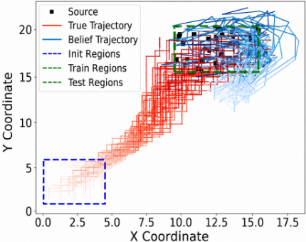
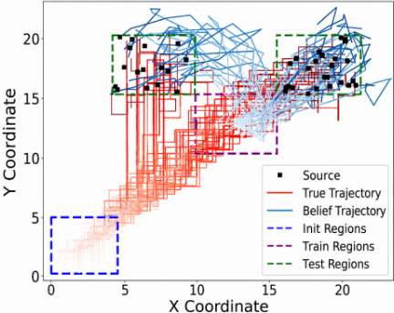
For out-of-distribution (OOD) experiments, the training region is confined to (10, 15) × (10, 15), while testing regions are (5, 10) × (15, 20) and (15, 20) × (15, 20) (Fig. 2b).
This spatially disjoint split evaluates whether policies rely on belief-conditioned decision rules rather than memorizing region-specific trajectories. Fields. We test seven field modalities: Temperature (Temp.), Concentration (Conc.), Magnetic (Mag.), Electric (Elec.), Gas (Gas), Energy (En.), and Noise (Noise), which differ in signal characteristics and noise patterns. Baselines. We compare against two groups: (i) RL+Bayes methods: AGDC-KLD [Shi et al., 2025] and its variants AGDC-ENT and AGDC-EE; (ii) planning+Bayes methods: Infotaxis [Vergassola et al., 2007], Entrotaxis [Hutchinson et al., 2018b], and DCEE [Chen et al., 2021]. A Random policy is included as a lower bound. Metrics. We report: (1) OCE (Operational Completion Efficacy), the stop rate under each method's stopping rule. For contraction-based methods, kstop is the first step satisfying ∥STDkstop ∥∞ < ζ (Sec. 4.3), otherwise kstop = Kmax, and OCE = Pr[kstop < Kmax]. (2) ADE (Average Deployment Efficiency), the traveled path length up to kstop, ADE = E[∑kstop-1 k=0 ∥pk+1 - pk∥2 ]. (3) LPS (Localization Precision Score), the terminal localization error of the posterior mean, LPS = E[∥(µxkstop , µykstop ) - (x∗ , y∗ )∥2 ]. We additionally report REV (runtime proxy; lower is faster) for completeness, but emphasize OCE/ADE/LPS for task performance.
5.2 Main results: in-distribution performance
| Method | Temp. | Conc. | Mag. | Elec. | Gas | En. | Noise |
|---|---|---|---|---|---|---|---|
| OCE | |||||||
| ATT-PFRL AGDC-KLD AGDC-ENT AGDC-EE Infotaxis Entrotaxis DCEE Random | 0.95±0.05 0.90±0.05 0.80±0.04 0.87±0.04 0.85±0.04 0.24±0.01 0.58±0.03 <0.05 | 0.94±0.05 0.91±0.05 0.81±0.04 0.88±0.04 0.86±0.04 0.23±0.01 0.59±0.03 | 0.94±0.05 0.89±0.04 0.81±0.04 0.86±0.04 0.85±0.04 0.25±0.01 0.58±0.03 <0.05 | 0.82±0.04 0.77±0.04 0.68±0.03 0.74±0.04 0.75±0.04 0.15±0.01 0.43±0.02 | 0.96±0.05 0.92±0.05 0.79±0.04 0.86±0.04 0.84±0.04 0.22±0.01 0.56±0.03 <0.05 | 0.63±0.03 0.61±0.03 0.51±0.03 0.57±0.03 0.55±0.03 0.14±0.01 0.36±0.02 <0.05 | 0.91±0.05 0.80±0.04 0.86±0.04 0.80±0.04 0.23±0.01 0.57±0.03 <0.05 |
| ATT-PFRL AGDC-KLD AGDC-ENT AGDC-EE Infotaxis Entrotaxis DCEE Random | 20±1.0 23±1.2 25±1.3 25±1.3 50±2.5 62±3.1 57±2.9 >150 | <0.05 19±1.0 22±1.1 24±1.2 24±1.2 48±2.4 60±3.0 55±2.8 >150 | 18±0.9 >150 <0.01 | <0.05 ADE 19±0.8 23±0.9 20±1.0 19±1.0 | 17±0.9 22±1.1 21±1.1 43±2.2 56±2.8 51±2.6 >150 | 19±0.5 22±0.6 24±0.7 0.09±0.05 0.07±0.04 0.07±0.04 0.07±0.04 0.80±0.04 0.70±0.04 0.70±0.04 <0.01 | 0.94±0.05 19±1.0 21±1.1 23±1.2 22±1.1 45±2.3 58±2.9 53±2.7 >150 |
| 23±0.7 58±1.9 47±1.4 | |||||||
| ATT-PFRL AGDC-ENT | 0.10±0.05 0.10±0.05 1.50±0.08 1.40±0.07 1.40±0.07 <0.01 0.05±0.01 0.20±0.01 | <0.01 | 22±1.1 25±1.2 24±1.2 51±2.4 59±3.0 54±2.7 | 61±2.5 55±2.3 >150 0.12±0.06 0.09±0.05 | 20±1.0 | 55±1.8 57±1.6 >150 | |
| 0.10±0.05 0.10±0.05 0.09±0.05 0.10±0.05 0.10±0.05 0.09±0.05 0.10±0.05 0.10±0.05 1.20±0.06 1.30±0.07 1.30±0.07 1.10±0.06 1.20±0.06 1.20±0.06 1.10±0.06 1.20±0.06 1.20±0.06 <0.01 <0.01 <0.01 LPS | |||||||
| AGDC-KLD AGDC-EE Infotaxis Entrotaxis DCEE Random | 0.10±0.05 | 0.10±0.05 0.10±0.05 0.10±0.05 1.40±0.07 1.30±0.07 1.30±0.07 | 0.14±0.07 | ||||
| REV | |||||||
| 0.15±0.08 | 0.14±0.07 | 0.14±0.07 0.10±0.05 0.10±0.05 0.10±0.05 1.40±0.07 | 0.13±0.07 | ||||
| 1.30±0.07 1.30±0.07 | |||||||
| ATT-PFRL AGDC-KLD AGDC-ENT AGDC-EE | |||||||
| 0.25±0.01 | 0.05±0.01 0.20±0.01 0.24±0.01 | 0.05±0.01 0.20±0.01 0.24±0.01 | 0.08±0.01 0.17±0.01 0.20±0.01 | 0.05±0.01 0.20±0.01 | 0.06±0.01 0.13±0.01 | 0.05±0.01 0.20±0.01 | |
| 0.22±0.01 | 0.18±0.01 | ||||||
| 0.22±0.01 | |||||||
| 0.23±0.01 | 0.20±0.01 | 0.14±0.01 0.12±0.01 | |||||
| 0.60±0.03 | 0.60±0.03 | 0.23±0.01 | |||||
| Infotaxis | 0.60±0.03 | 0.60±0.03 | 0.51±0.02 | 0.39±0.02 | |||
| 0.22±0.01 | |||||||
| 0.21±0.01 | |||||||
| Entrotaxis DCEE Random | 0.70±0.04 0.60±0.03 5.0±0.25 | 0.70±0.04 0.60±0.03 5.0±0.25 | 0.70±0.04 0.60±0.03 5.0±0.25 | 0.60±0.03 0.51±0.02 5.0±0.25 | 0.70±0.04 0.60±0.03 5.0±0.25 | 0.46±0.02 0.39±0.02 5.0±0.25 | 0.60±0.03 0.70±0.04 0.60±0.03 5.0±0.25 |
Table 2 provides end-to-end evidence that ATT-PFRL improves both task completion and localization accuracy across all field modalities. High OCE indicates that the learned policy can reliably trigger termination, while low LPS indicates that termination typically occurs near the true source rather than due to accidental contraction.The large ADE gap vs. planning baselines suggests that hand-crafted heuristics can be myopic under noise/model mismatch, while beliefconditioned RL learns more efficient information gathering.
5.3 Generalization: out-of-distribution
| Method | Temp. | Conc. | Mag. | Elec. | Gas | En. | Noise |
|---|---|---|---|---|---|---|---|
| ATT-PFRL (ours) | 0.95 | 0.94 | 0.94 | 0.82 | 0.96 | 0.63 | 0.94 |
| AGDC-KLD | 0.448 | 0.453 | 0.446 | 0.382 | 0.458 | 0.307 | 0.452 |
| AGDC-ENT | 0.271 | 0.268 | 0.273 | 0.225 | 0.265 | 0.168 | 0.269 |
| AGDC-EE | 0.288 | 0.291 | 0.285 | 0.249 | 0.289 | 0.192 | 0.285 |
Table 3: OOD generalization across fields (spatially shifted regions)
OOD performance drops substantially for RL+Bayes baselines, while ATT-PFRL maintains high completion rates across fields (Table 3). Fig. 2b further shows that belief trajectories continue to converge near the source under spatial shifts, providing a process-level explanation for the aggregated OCE results. Since OOD amplifies inference errors, we next test inference robustness via fixed-trajectory evaluation.
5.4 Uniformmixing lacks attention
Uniform mixing is a special case of convex smoothing on the weight simplex: ˜wi = (1-ρ)wi +ρ 1N , ρ ∈ [0, 1], which corresponds to replacing feature-aware attention with a uniform row-stochastic matrix. We test whether the gain of attention is merely due to generic smoothing by sweeping ρ.
| ρ | ADE (Basic) | OCE (Basic) | ADE (OOD) | OCE (OOD) |
|---|---|---|---|---|
| 0.0 | 22±1.1 | 0.93±0.05 | 28±1.4 | 0.88±0.04 |
| 0.1 | 19±1.0 | 0.95±0.05 | 24±1.2 | 0.91±0.05 |
| 0.2 | 18±0.9 | 0.96±0.05 | 23±1.2 | 0.92±0.05 |
| 0.3 | 20±1.0 | 0.94±0.05 | 26±1.3 | 0.89±0.04 |
| 0.4 | 25±1.3 | 0.90±0.05 | 32±1.6 | 0.84±0.04 |
| 0.5 | 32±1.6 | 0.85±0.04 | 40±2.0 | 0.78±0.04 |
| Convex | Non-convex | ||||||
|---|---|---|---|---|---|---|---|
| Dist. | OCE | ADE | LPS | Dist. | OCE | ADE | LPS |
| Beta | 0.95±0.05 | 19±1.0 | 0.05±0.01 | Star Shape | 0.92±0.05 | 22±1.1 | 0.07±0.01 |
| Gaussian | 0.96±0.05 | 18±0.9 | 0.04±0.01 | Quarter Ring | 0.90±0.05 | 24±1.2 | 0.08±0.01 |
| Dirichlet | 0.94±0.05 | 20±1.0 | 0.06±0.01 | Half Ring | 0.88±0.04 | 26±1.3 | 0.09±0.01 |
| Uniform | 0.95±0.05 | 19±1.0 | 0.05±0.01 | Full Ring | 0.86±0.04 | 28±1.4 | 0.10±0.01 |
Table 4 shows a sweet-spot behavior: mild uniform mixing (ρ ≈ 0.1-0.2) slightly improves OCE/ADE by mitigating extreme collapse, but larger ρ biases the posterior toward uniformity and degrades both ID and OOD performance. This control rules out the alternative explanation that "any smoothing" would work; the benefit comes from feature-aware mass transfer that preserves informative modes. Table 5 further demonstrates robustness to prior-shape mismatch (including non-convex priors), supporting that attention regularization does not rely on a fortunate prior geometry and remains stable under diverse belief initializations.
5.5 Adaptation under nonstationary source shifts
We evaluate adaptability in a nonstationary setting where the source location undergoes an abrupt change during inference: after 15 steps, the source position shifts to a new location while the agent continues operating without reset. This tests whether the inference layer can rapidly reallocate posterior mass after a regime change.
| Field | OCE | ADE | LPS | |||
|---|---|---|---|---|---|---|
| Ours | AGDC-KLD | Ours | AGDC-KLD | Ours | AGDC-KLD | |
| Temperature | 0.95±0.05 | 0.90±0.05 | 20±1.0 | 23±1.2 | 0.05±0.01 | 0.20±0.01 |
| Concentration | 0.94±0.05 | 0.91±0.05 | 19±1.0 | 22±1.1 | 0.05±0.01 | 0.20±0.01 |
| Magnetic | 0.94±0.05 | 0.89±0.04 | 18±0.9 | 22±1.1 | 0.05±0.01 | 0.20±0.01 |
| Electric | 0.82±0.04 | 0.77±0.04 | 19±0.8 | 23±0.9 | 0.08±0.01 | 0.17±0.01 |
| Gas | 0.96±0.05 | 0.92±0.05 | 17±0.9 | 20±1.0 | 0.05±0.01 | 0.20±0.01 |
| Energy | 0.63±0.03 | 0.61±0.03 | 19±0.5 | 22±0.6 | 0.06±0.01 | 0.13±0.01 |
| Noise | 0.94±0.05 | 0.91±0.05 | 19±1.0 | 21±1.1 | 0.05±0.01 | 0.20±0.01 |
Nonstationarity is a stricter stress test than spatial OOD: the agent must abandon an already contracting belief and relocalize without resetting exploration. ATT-PFRL maintains higher completion and lower localization error than AGDCKLD, suggesting that degeneracy control and rejuvenation help preserve particle diversity, which in turn enables faster posterior reallocation after regime changes. This observation is consistent with the fixed-trajectory results in Sec. 5.6: higher ESS correlates with stronger recovery from weak or shifting observations in Table 6.
5.6 Inference ablation: fixed-trajectory evaluation
| Method | RMSE@20 (m)↓ | ESS@20↑ | Likelihood Evals↓ | Wall-time (ms)↓ |
|---|---|---|---|---|
| PF-baseline | 5.2±0.8 | 120±35 | 10000 | 45±8 |
| PF+Attention (R=0) | 3.6±0.6 | 240±50 | 10500 | 52±9 |
| PF+MH (ε=0) | 4.1±0.7 | 180±42 | 15000 | 68±12 |
| PF+Att+MH (Ours) | 2.8±0.4 | 285±48 | 15800 | 72±11 |
To isolate the contribution of the inference layer (ESStriggered resampling, feature-aware attention smoothing, and MH rejuvenation) from policy-induced data collection, we compare inference variants under identical observation sequences o1:K. We evaluate on the most challenging setting: fixed random-walk trajectories where observations are weakly informative. Table 7 shows that attention smoothing substantially increases ESS and reduces RMSE, indicating that it directly mitigates weight collapse. MH rejuvenation alone yields a smaller gain, while combining attention and MH achieves the best RMSE/ESS, supporting the complementarity claimed in Sec. 4.2: attention prevents extreme collapse, and MH restores diversity after resampling. This provides a causal explanation for the end-to-end improvements in Table 2 and the robustness observed under OOD tests.
5.7 Cessation & reward validation
Our framework uses belief contraction both as a termination criterion and as an intrinsic learning signal: termination occurs when ∥STDk∥∞ < ζ, and rk+1 = I[∥STDk+1∥∞ < ζ]. This subsection validates (i) threshold sensitivity, (ii) calibration against ground-truth accuracy, and (iii) reward design.
Threshold sensitivity with GT-success. To avoid circular evaluation (defining success using the same threshold being swept), we evaluate termination using an independent ground-truth criterion: let estop = ∥(µx, µy) - (x⋆ , y⋆ )∥2 at termination and define GT-success as estop < ϵloc with ϵloc = 1.0m. We sweep ζ only at test time, keeping policy and inference fixed.
| ζ | Stop Rate ↑ | GT-Success ↑ | Avg. Steps ↓ | ADE ↓ | False Stop ↓ |
|---|---|---|---|---|---|
| 0.2 | 0.88 | 0.96 | 31±6 | 22±2 | 0.02 |
| 0.3 | 0.92 | 0.95 | 28±5 | 21±2 | 0.04 |
| 0.4 | 0.94 | 0.94 | 24±4 | 20±1 | 0.06 |
| 0.5 | 0.95 | 0.92 | 22±4 | 20±1 | 0.08 |
| 0.6 | 0.96 | 0.89 | 20±3 | 19±1 | 0.12 |
| 0.7 | 0.97 | 0.86 | 18±3 | 19±2 | 0.15 |
| 0.8 | 0.98 | 0.81 | 16±3 | 18±2 | 0.21 |
| 1.0 | 0.99 | 0.75 | 14±2 | 18±2 | 0.28 |
As ζ increases, Stop Rate rises monotonically, but GTSuccess decreases and False Stop increases, revealing a clear efficiency-accuracy trade-off. The default ζ = 0.5 is a balanced operating point: it achieves strong GT-Success while avoiding excessive exploration (Table 8). This directly supports the claim that our stopping signal is not only effective (high OCE) but also controllable and transferable.
Calibration against ground-truth error. On 1,000 test episodes per field, we record contraction ck = ∥STDk∥∞ and ground-truth error ek over time. We report Spearman rank correlation, false termination rate at ζ = 0.5, and precision/recall of I[ck < ζ]. The contraction signal is consistently and strongly negatively correlated with true localization error across all fields, indicating that posterior contraction is a reliable proxy for accuracy rather than an arbitrary confidence measure. Importantly, this calibration becomes meaningful in light of Sec. 5.6: since the inference layer demonstrably improves RMSE/ESS under controlled observations, the contraction signal is grounded in improved posterior quality, mitigating "confident but wrong" failure modes.
| Criterion | GT-Success ↑ | Avg. Steps ↓ | False Term. ↓ | ρS ↓ |
|---|---|---|---|---|
| ∥STD∥∞ < 0.5 (ours) | 0.92 | 22±4 | 0.08 | -0.78 |
| Entropy < τH | 0.87 | 24±5 | 0.14 | -0.68 |
| maxi wi > τw | 0.84 | 20±4 | 0.18 | -0.61 |
| Fixed steps (k=25) | 0.79 | 25 | 0.23 | N/A |
We compare contraction-based cessation with entropy thresholding, max-weight thresholding, and fixed-step stopping on Temperature (ID) in Table 9. This comparison shows that contraction-based cessation achieves the best overall balance: it yields higher GT-Success and lower premature termination than entropy/max-weight criteria.
| Reward Type | OCE (ID) ↑ | GT-Success (ID) ↑ | ADE ↓ | OCE (OOD) ↑ | Sample Eff. ↓ |
|---|---|---|---|---|---|
| R1: Indicator (ours) | 0.95 | 0.92 | 20±1 | 0.88 | 1200 eps to 0.90 |
| R2: Dense contraction | 0.91 | 0.87 | 21±1 | 0.84 | 980 eps to 0.90 |
| R3: Entropy reduction | 0.88 | 0.83 | 23±1 | 0.80 | 1450 eps to 0.90 |
Reward formulation ablation. We train ATT-PFRL under three intrinsic reward variants with identical budgets: (R1) indicator (ours), (R2) dense contraction shaping, and (R3) entropy reduction in Table 10. Dense shaping (R2/R3) can speed up early learning but degrades asymptotic performance and OOD generalization, suggesting that optimizing a dense proxy (contraction reduction per step) can misalign the policy with the actual stopping objective. In contrast, the indicator reward (R1) directly matches the cessation goal and therefore preserves goal alignment under shifts, closing the loop between inference quality (Sec. 5.6), and robust end-to-end behavior (Secs. 5.2-5.3).
6 Conclusion
We present ATT-PFRL for active source localization under sparse feedback by coupling belief inference with RL. The attention-augmented particle filter mitigates degeneracy and improves posterior quality. Experiments across diverse fields show higher completion and better localization than RL+Bayes and planning baselines, including OOD. Belief contraction is calibrated as a stopping signal and provides an intrinsic reward without hand-crafted distance shaping.
@inproceedings{ijcai2026p726,
  title     = {Belief-Contraction-Driven Active Inverse Source Localization and Characterization},
  author    = {Shi, Yiwei and Yang, Mengyue and Zhang, Qi and Liu, Cunjia and Zhang, Weinan and Liu, Weiru},
  booktitle = {Proceedings of the Thirty-Fifth International Joint Conference on
               Artificial Intelligence, {IJCAI-26}},
  publisher = {International Joint Conferences on Artificial Intelligence Organization},
  editor    = {Diego Calvanese},
  pages     = {6528--6535},
  year      = {2026},
  month     = {8},
  note      = {AI4Tech: AI Enabling Technologies},
  doi       = {10.24963/ijcai.2026/726},
  url       = {https://doi.org/10.24963/ijcai.2026/726},
}
TY - CPAPER TI - Belief-Contraction-Driven Active Inverse Source Localization and Characterization AU - Shi, Yiwei AU - Yang, Mengyue AU - Zhang, Qi AU - Liu, Cunjia AU - Zhang, Weinan AU - Liu, Weiru T2 - Proceedings of the Thirty-Fifth International Joint Conference on Artificial Intelligence, IJCAI-26 PB - International Joint Conferences on Artificial Intelligence Organization PY - 2026 SP - 6528 EP - 6535 DO - 10.24963/ijcai.2026/726 UR - https://doi.org/10.24963/ijcai.2026/726 ER -Copied
Machine-readable versions of this paper, for tools and AI agents:





