
DUALFloodGNN: Physics-informed Graph Neural Network for Operational Flood Modeling
Proceedings of the Thirty-Fifth International Joint Conference on Artificial Intelligence. AI4Tech: AI Enabling Technologies. Pages 6408-6416.
https://doi.org/10.24963/ijcai.2026/713
Keywords
- Domain-specific AI4Tech: AI4Home and AI4City
- AI4Tech infrastructure/systems: AI social systems
- Domain-specific AI4Tech: AI4Safety
- Advanced AI4Tech: Deep AI4Tech
- Advanced AI4Tech: Data-driven AI4Tech
Abstract
Flood models inform strategic disaster management by simulating the spatiotemporal hydrodynamics of flooding. While physics-based numerical flood models are accurate, their substantial computational cost limits their use in operational settings where rapid predictions are essential. Models designed with graph neural networks (GNNs) provide both speed and accuracy while having the ability to process unstructured spatial domains. Given its flexible input and architecture, GNNs can be leveraged alongside physics-informed techniques with ease, significantly improving interpretability and generalizability. We introduce a novel flood GNN architecture, DUALFloodGNN, which embeds physical constraints at both global and local scales through explicit loss terms. The model jointly predicts water volume at nodes and flow along edges through a shared message-passing framework. To improve performance for autoregressive inference, model training is conducted with a multi-step loss enhanced with dynamic curriculum learning. Compared with standard GNN architectures and state-of-the-art GNN flood models, DUALFloodGNN achieves substantial improvements in predicting multiple hydrologic variables (e.g., water volume, flow, and depth) while maintaining high computational efficiency. The model is open sourced at https://github.com/acostacos/dual_flood_gnn. The dataset is open sourced at https://doi.org/10.25910/9xav-0s86.
- Model RMSE () ↓ MAE (m 3 ) ↓ GCN (node) 9,849.98 ± 2,485.73 6,340.51 ± 1,859.60 GAT (node) 13,232.86 ± 11,835.18 4,583.68 ± 1,969.27 GraphSAGE (node) 11,146.97 ± 11,420.79 4,177.75 ± 2,519.14 GIN (node) 5,023.18 ± 1,450.37 2,587.05 ± 798.38 GINE (node) 3,437.68 ± 693.94 1,860.03 ± 406.78 HydroGraphNet 7,584.51 ± 3,068.54 3,343.52 ± 1,392.34 DUALFloodGNN 2,216.27 ± 868.21 1,075.63 ± 394.
- [Ahmadlou et al., 2021] Mohammad Ahmadlou, A'kif Al- Fugara, Abdel Rahman Al-Shabeeb, Aman Arora, Rida Al-Adamat, Quoc Bao Pham, Nadhir Al-Ansari, Nguyen Thi Thuy Linh, and Hedieh Sajedi. Flood susceptibil- ity mapping and assessment using a novel deep learning model combining multilayer perceptron and autoencoder neural networks. Journal of Flood Risk Management, 14(1):e12683, 2021.
- [Ashraf et al., 2024] Inaam Ashraf, Janine Strotherm, Luca Hermes, and Barbara Hammer. Physics-informed graph neural networks for water distribution systems. Proceed- ings of the AAAI Conference on Artificial Intelligence, 38(20):21905-21913, 3 2024.
- [Battaglia et al., 2018] Peter W. Battaglia, Jessica B. Ham- rick, Victor Bapst, Alvaro Sanchez-Gonzalez, Vinicius Zambaldi, Mateusz Malinowski, Andrea Tacchetti, David Raposo, Adam Santoro, Ryan Faulkner, Caglar Gulcehre, Francis Song, Andrew Ballard, Justin Gilmer, George Dahl, Ashish Vaswani, Kelsey Allen, Charles Nash, Vic- toria Langston, Chris Dyer, Nicolas Heess, Daan Wierstra, Pushmeet Kohli, Matt Botvinick, Oriol Vinyals, Yujia Li, and Razvan Pascanu. Relational inductive biases, deep learning, and graph networks, 2018.
- [Bentivoglio et al., 2023] R. Bentivoglio, E. Isufi, S. N. Jonkman, and R. Taormina. Rapid spatio-temporal flood modelling via hydraulics-based graph neural networks. Hydrology and Earth System Sciences, 27(23):4227-4246, 2023.
- [Bentivoglio et al., 2024] R. Bentivoglio, E. Isufi, S. N. Jonkman, and R. Taormina. Multi-scale hydraulic graph neural networks for flood modelling. EGUsphere, 2024:1- 28, 2024.
- [Bronstein et al., 2017] Michael M. Bronstein, Joan Bruna, Yann LeCun, Arthur Szlam, and Pierre Vandergheynst. Geometric deep learning: Going beyond euclidean data. IEEE Signal Processing Magazine, 34(4):18-42, July 2017.
- [Brunner, 2025] Gary W. Brunner. HEC-RAS Hydraulic Ref- erence Manual. Hydrologic Engineering Center, Insti- tute for Water Resources, U.S. Army Corps of Engineers, 2025. Accessed: 2025-12-16.
- [Costabile et al., 2017] Pierfranco Costabile, Carmelina Costanzo, and Francesco Macchione. Performances and limitations of the diffusive approximation of the 2-d shallow water equations for flood simulation in urban and rural areas. Applied Numerical Mathematics, 116:141- 156, 2017. New Trends in Numerical Analysis: Theory, Methods, Algorithms and Applications (NETNA 2015).
- [Devia et al., 2015] Gayathri K. Devia, B.P. Ganasri, and G.S. Dwarakish. A review on hydrological models. Aquatic Procedia, 4:1001-1007, 2015. International Con- ference on Water Resources, Costal AND Ocean Engineer- ing (ICWRCOE'15).
- [Fang et al., 2021] Zhice Fang, Yi Wang, Ling Peng, and Haoyuan Hong. Predicting flood susceptibility using lstm neural networks. Journal of Hydrology, 594:125734, 2021.
- [Farahmand et al., 2023] Hamed Farahmand, Yuanchang Xu, and Ali Mostafavi. A spatial-temporal graph deep learning model for urban flood nowcasting leveraging heterogeneous community features. Scientific Reports, 13(1):6768, 4 2023.
- [Fey and Lenssen, 2019] Matthias Fey and Jan Eric Lenssen. Fast graph representation learning with pytorch geometric, 2019.
- [Gao et al., 2022] Han Gao, Matthew J. Zahr, and Jian-Xun Wang. Physics-informed graph neural galerkin networks: A unified framework for solving pde-governed forward and inverse problems. Computer Methods in Applied Me- chanics and Engineering, 390:114502, 2022.
- [Gilmer et al., 2017] Justin Gilmer, Samuel S. Schoenholz, Patrick F. Riley, Oriol Vinyals, and George E. Dahl. Neural message passing for quantum chemistry, 2017.
- [Hamilton et al., 2018] William L. Hamilton, Rex Ying, and Jure Leskovec. Inductive representation learning on large graphs, 2018.
- [Herath et al., 2025] Herath Mudiyanselage Viraj Vidura Herath, Lucy Marshall, Abhishek Saha, Sanka Rasnayaka, and Sachith Seneviratne. Subgrid informed neural net- works for high-resolution flood mapping. Journal of Hy- drology, 660, 10 2025.
- [Hosseiny, 2021] Hossein Hosseiny. A deep learning model for predicting river flood depth and extent. Environmental Modelling & Software, 145:105186, 2021.
- [Hu et al., 2020] Weihua Hu, Bowen Liu, Joseph Gomes, Marinka Zitnik, Percy Liang, Vijay Pande, and Jure Leskovec. Strategies for pre-training graph neural net- works, 2020.
- [Jiang et al., 2019] Xiaodong Jiang, Pengsheng Ji, and Sheng Li. Censnet: Convolution with edge-node switch- ing in graph neural networks. In Proceedings of the Twenty-Eighth International Joint Conference on Artifi- cial Intelligence, IJCAI-19, pages 2656-2662. Interna- tional Joint Conferences on Artificial Intelligence Orga- nization, 7 2019. IJCAI
- [Jiang et al., 2024] Jiange Jiang, Chen Chen, Yang Zhou, Stefano Berretti, Lei Liu, Qingqi Pei, Jianming Zhou, and Shaohua Wan. Heterogeneous dynamic graph convolu- tional networks for enhanced spatiotemporal flood fore- casting by remote sensing. IEEE Journal of Selected Top- ics in Applied Earth Observations and Remote Sensing, 17:3108-3122, 2024.
- [Kazadi et al., 2024] Arnold Kazadi, James Doss-Gollin, Antonia Sebastian, and Arlei Silva. Floodgnn-gru: a spatio-temporal graph neural network for flood prediction. Environmental Data Science, 3:e21, 2024.
- [Kipf and Welling, 2017] Thomas N. Kipf and Max Welling. Semi-supervised classification with graph convolutional networks, 2017.
- [Kumar et al., 2023] Vijendra Kumar, Kul Vaibhav Sharma, Tommaso Caloiero, Darshan J. Mehta, and Karan Singh. Comprehensive overview of flood modeling approaches: A review of recent advances. Hydrology, 10(7), 2023.
- [Luo et al., 2024] Yuxuan Luo, Yanlai Zhou, Hua Chen, Li- hua Xiong, Shenglian Guo, and Fi-John Chang. Exploring a spatiotemporal hetero graph-based long short-term mem- ory model for multi-step-ahead flood forecasting. Journal of Hydrology, 633:130937, 2024.
- [Neo et al., 2025] Sun Han Neo, Sachith Seneviratne, Herath Mudiyanselage Viraj Vidura Herath, Abhishek Saha, Sanka Rasnayaka, and Lucy Amanda Marshall. Flood- ldm: Generalizable latent diffusion models for rapid and accurate zero-shot high-resolution flood mapping, 2025.
- [Oliveira Santos et al., 2023] Victor Oliveira Santos, Paulo Alexandre Costa Rocha, John Scott, Jesse Van Griensven Thé, and Bahram Gharabaghi. A new graph-based deep learning model to predict flooding with validation on a case study on the humber river. Water, 15(10), 2023.
- [Rahimzad et al., 2021] M. Rahimzad, A. Moghaddam Nia, H. Zolfonoon, et al. Performance comparison of an lstm- based deep learning model versus conventional machine learning algorithms for streamflow forecasting. Water Re- sources Management, 35(12):4167-4187, 2021.
- [Rentschler et al., 2022] Jun Rentschler, Melda Salhab, and Bramka Arga Jafino. Flood exposure and poverty in 188 countries. Nature Communications, 13(1):3527, 6 2022.
- [Roudbari et al., 2024] Naghmeh Shafiee Roudbari, Shub- ham Rajeev Punekar, Zachary Patterson, Ursula Eicker, and Charalambos Poullis. From data to action in flood forecasting leveraging graph neural networks and digi- tal twin visualization. Scientific Reports, 14(1):18571, 8 2024.
- [Sharma et al., 2023] Pushan Sharma, Wai Tong Chung, Bassem Akoush, and Matthias Ihme. A review of physics- informed machine learning in fluid mechanics. Energies, 16(5), 2023.
- [Sun et al., 2023] Alexander Y. Sun, Zhi Li, Wonhyun Lee, Qixing Huang, Bridget R. Scanlon, and Clint Dawson. Rapid flood inundation forecast using fourier neural op- erator, 2023.
- [Tabari, 2020] Hossein Tabari. Climate change impact on flood and extreme precipitation increases with water avail- ability. Scientific Reports, 10(1):13768, 2020.
- [Taghizadeh et al., 2025] Mohammad Taghizadeh, Zahra Zandsalimi, Mohammad Amin Nabian, Majid Shafiee- Jood, and Negin Alemazkoor. Interpretable physics- informed graph neural networks for flood forecasting. Computer-Aided Civil and Infrastructure Engineering, pages 1-21, 2025.
- [Teutsch and Mäder, 2022] Philipp Teutsch and Patrick Mäder. Flipped classroom: Effective teaching for time series forecasting, 2022. [Thangamuthu et al., 2023]
- Abishek Thangamuthu, Gunjan Kumar, Suresh Bishnoi, Ravinder Bhattoo, N M Anoop Krishnan, and Sayan Ranu. Unravelling the performance of physics-informed graph neural networks for dynamical systems, 2023. [UNDRR and CRED, 2020] UNDRR and CRED. The Hu- man Cost of Disasters: An Overview of the Last 20 Years (2000-2019), 10 2020.
- [Veličković et al., 2018] Petar Veličković, Guillem Cucurull, Arantxa Casanova, Adriana Romero, Pietro Liò, and Yoshua Bengio. Graph attention networks, 2018.
- [Xie et al., 2021] Shuai Xie, Wenyan Wu, Sebastian Mooser, Q.J. Wang, Rory Nathan, and Yuefei Huang. Artificial neural network based hybrid modeling approach for flood inundation modeling. Journal of Hydrology, 592:125605, 2021.
- [Xu et al., 2019] Keyulu Xu, Weihua Hu, Jure Leskovec, and Stefanie Jegelka. How powerful are graph neural net- works?, 2019.
- [Yang and Li, 2020] Yulei Yang and Dongsheng Li. Nenn: Incorporate node and edge features in graph neural net- works. In Sinno Jialin Pan and Masashi Sugiyama, edi- tors, Proceedings of The 12th Asian Conference on Ma- chine Learning, volume 129 of Proceedings of Machine Learning Research, pages 593-608. PMLR, 11 2020.
- [Zhang et al., 2024] Zhiyu Zhang, Wenchong Tian, Chenkaixiang Lu, Zhenliang Liao, and Zhiguo Yuan. Graph neural network-based surrogate modelling for real-time hydraulic prediction of urban drainage networks. Water Research, 263:122142, 2024.
- [Zhao et al., 2020] Qun Zhao, Yuelong Zhu, Kai Shu, Ding- sheng Wan, Yufeng Yu, Xudong Zhou, and Huan Liu. Joint spatial and temporal modeling for hydrological prediction. IEEE Access, 8:78492-78503, 2020.
References were extracted automatically from the PDF and may contain errors.
Full text extracted automatically from the PDF; figures, tables and equations may differ. The PDF is the version of record.
1 Introduction
Floods pose a substantial socioeconomic threat to modern society, resulting in losses of more than 3 trillion USD in the past 25 years and affecting up to 1.81 billion individuals globally [Rentschler et al., 2022; UNDRR and CRED, 2020]. Furthermore, the frequency and severity of such events are only projected to increase due to climate change [Tabari, 2020]. Effective mitigation of these repercussions requires detailed flood information. In such cases, hydrodynamic flood models play a crucial role by simulating water behavior across space and time, enabling data-driven disaster management and flood-resilient engineering designs [Kumar et al., 2023]. Conventional physics-based numerical models capture flood dynamics with high accuracy by solving the governing equations of fluid flow. However, they require substantial computation time, limiting their effectiveness for real-time or operational use [Sun et al., 2023].
To address this, data-driven surrogate models forecast flooding through statistical correlations, resulting in much faster computation speed. In particular, deep learning (DL) has the ability to automatically learn and extract complex non-linear relationships from data, making it suitable for modeling flood movement. Research continues to assess the efficacy of various architectures including multilayer perceptrons (MLPs) [Ahmadlou et al., 2021; Xie et al., 2021], recurrent neural networks (RNNs) [Fang et al., 2021; Rahimzad et al., 2021] and convolutional neural networks (CNNs) [Herath et al., 2025; Hosseiny, 2021; Neo et al., 2025]. Although suitable for real-time forecasting, DL models are often criticized as "black boxes", due to a limited understanding of their predictive paradigm [Devia et al., 2015]. Such an opacity presents a significant disadvantage in physics-based disciplines, where explainability is essential to ensure consistency with physical laws.
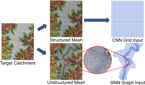
Physics-informed DL models combine the strengths of data-driven and physics-based approaches by embedding physical constraints into DL architectures, enabling them to learn the underlying behavior of physical systems [Sharma et al., 2023]. The main challenge of this approach lies in the complexity of aligning existing algorithms in both domains. An example of such a case is illustrated in figure 1. Physicsbased numerical approximations involve the discretization of the area into a mesh structure, which is typically integrated in DL models through CNNs, given their aptitude with spatial input [Gao et al., 2022]. However, this methodology is also fundamentally constrained by the nature of CNNs, which are restricted to processing structured grid meshes. This limits physical fidelity, as this discretization scheme cannot adequately represent the irregular topographies and nonuniform fluid dynamics characteristic of flooding scenarios. Graph neural networks (GNNs) were developed to directly address this limitation by generalizing CNN-based convolution for arbitrary spatial data represented as graphs [Bronstein et al., 2017]. This representation enables a more flexible description of hydrodynamic quantities through an unstructured mesh and has been shown to improve generalization in physical systems [Thangamuthu et al., 2023].
Integration of physics-informed techniques with GNN flood models is still an emerging field of research. For example, HydroGraphNet [Taghizadeh et al., 2025] incorporates the principle of mass conservation at a global graphlevel through a regularization term in the loss function. However, local mass conservation is only implicitly assumed, as global mass balance does not guarantee the same behavior in smaller regions. We address this research gap by incorporating an additional loss term explicitly promoting nodelevel mass balance. To enable this, we diverge from previous approaches [Bentivoglio et al., 2023; Bentivoglio et al., 2024] by mapping the time-varying water flow as an edge attribute, thus preserving its vector characteristics. This graph mapping provides more intuitive physical meaning, and closely mimics the capabilities of physics-based numerical models. However, this also introduces the challenge of predicting both node and edge features. Existing domainagnostic GNNs created for this purpose [Jiang et al., 2019; Yang and Li, 2020] require the generation of a line graph, which typically contains more nodes and edges, increasing computational overhead. We develop a novel architecture that performs simultaneous node and edge prediction given only the original graph utilizing two separate decoders. We coin our approach Double-target Universally And Locally constrained Flood GNN (DUALFloodGNN).
Our contributions can be summarized as follows:
- We develop a physics-informed loss function that promotes mass conservation at both global and local scales through multiple regularization terms, preserving conservation within localized areas of the computational mesh and ensuring physically realistic flood dynamics.
- To facilitate the computation of local mass balance, we design an architecture capable of simultaneously predicting features for nodes (water volume) and edges (wa-
- ter flow). Joint modeling is performed through shared message generation, which utilizes their physical correlation while requiring only the original graph structure.
- To the best of our knowledge, this is the first study to benchmark performance across different GNN-based flood models. Experimental results validate the effectiveness of DUALFloodGNN, which outperforms both standard GNN baselines and state-of-the-art GNN flood models [Bentivoglio et al., 2023; Taghizadeh et al., 2025].
2 Background and RelatedWork
Graph Neural Networks. GNNs have found widespread use in the processing of graph-structured data [Hamilton et al., 2018; Kipf and Welling, 2017; Veliˇckovi´c et al., 2018]. GNNs generalize CNN-based convolution for non-Euclidean domains [Bronstein et al., 2017] through the message passing framework [Gilmer et al., 2017]. Given a node i in the graph, its node embedding hli for the current layer l is updated to hl+1 i based on its local neighborhood N(i) through Eq. 1:
where hj are the neighbor embeddings and M, A and U are the message, aggregate and update functions. This is repeated for each node in the graph, creating an updated graph representation after one full cycle. Each layer in a GNN corresponds to one message passing iteration, which can be repeated to enable further message propagation.
Node and Edge Prediction. Convolution with edge-node switching network (CensNet) [Jiang et al., 2019] learns both node- and edge-level features through alternating spectral graph convolutions using the original graph for node embeddings and the line graph for edge embeddings. Node and Edge Neural Network (NENN) [Yang and Li, 2020] extends this approach to spatial-based message passing and incorporates attention to both node- and edge-level layers.
GNNs for Flood Modeling. Initial studies adopted existing architectures for the hydrological context [Farahmand et al., 2023; Oliveira Santos et al., 2023]. Further studies incorporated RNN components to explicitly capture the temporal aspect of flood dynamics [Kazadi et al., 2024; Roudbari et al., 2024; Zhao et al., 2020], with some utilizing heterogeneous graph structures to encode diverse relationships within the system [Jiang et al., 2024; Luo et al., 2024].
Physics-informed Flood GNNs. Physics-informed constraints were integrated either through the model architecture or loss function. ShallowWater Equation-Graph Neural Network (SWE-GNN) [Bentivoglio et al., 2023] modulates propagated messages by the latent gradient between neighboring nodes, which is extended for a multi-scale architecture in multi-scale SWE-GNN (mSWE-GNN) [Bentivoglio et al., 2024]. GNN-fusion [Zhang et al., 2024] computes flow at a node as the sum of predicted flow from its adjacent edges to reliably enforce mass conservation. While it supports node and edge prediction, their model generates these embeddings with different convolutions and has only been tested for 1D flow in drainage networks. HydroGraphNet [Taghizadeh et al., 2025] introduces a physics-based loss that encourages global mass conservation through a forward and backward check, ensuring the predicted water volume is within bounds.
3 Preliminaries
Notations. Formally, a graph G = (V, E) is comprised of a set of nodes V and edges E. Nodes are described by a node feature matrix X = R|V|×fv where fv is the node feature dimension. Edges are typically represented in terms of an adjacency matrix A ∈ {0, 1}|V|×|V| where Aij = 1 if a connecting edge exists from node i to node j, otherwise, Aij = 0. A memory-efficient alternative, especially for sparse graphs, is the coordinate (COO) format I = R2×|E| where (i, j) ∈ I if there is an edge from node i to node j [Fey and Lenssen, 2019]. Through this representation, edges can be described with multi-dimensional feature vectors, which combine to form the edge feature matrix E = R|E|×fe where fe is the edge feature dimension.
ProblemDefinition. A flood event is represented as a time series of directed graphs {G0,G1, ...,GT} where nodes and edges have associated water volume (V ) and flow ( ⃗Q) values respectively. Water flow is a vector quantity where ⃗Q > 0 denotes flow along the edge's orientation and ⃗Q < 0 indicates movement in the opposite direction. Nodes and edges can be further described by static structural properties of the catchment. The model performs a node- and edge-level regression task to predict future hydraulic states {V t+n , ⃗Qt+n |n = 1, ..., T} at each structure given the initial state at the current timestep t and up to p previous states {V t-n , ⃗Qt-n |n = 0, ..., p}. Predictions are obtained in an autoregressive manner, where the predicted features are used recursively as dynamic features for subsequent model inference. Additionally, boundary conditions (e.g., rainfall R, upstream inflow ⃗Qin and downstream outflow ⃗Qout) are supplied at each timestep {Rt+n , ⃗Qt+n in , ⃗Qt+n out |n = 0, ..., T -1}, describing water flow entering and exiting the system.
4 Methodology
Overview. In this section, we discuss DUALFloodGNN, a novel physics-informed GNN architecture used for the simultaneous prediction of node water volume and edge water flow. It is comprised of three main components: (1) a model that performs shared message passing to predict both node and edge features, (2) a physics-informed loss function that enforces global and local mass conservation between consecutive predictions, and (3) an autoregressive training strategy utilizing dynamic curriculum learning. Figure 2 provides a diagram illustrating this framework.
4.1 Model Architecture
Input and Output. The input of the model is a directed graph at timestep t containing static features (e.g., area, elevation) and dynamic features (e.g., volume, flow, rainfall, global inflow) up to p previous timesteps. The node and edge feature matrices Xt and Et are created through Eq. 2 and Eq. 3:
where || is the concatenation operation. Instead of predicting future states directly, DUALFloodGNN predicts the change in water volume ∆V and water flow ∆⃗Q from the current timestep to the next timestep. This reduces the variation in the output, achieving more stable and accurate long-horizon predictions. The model's prediction can be added to the current dynamic features V t and ⃗Qt to get the next timestep values V t+1 and ⃗Qt+1 , which also acts as a residual connection.
To facilitate joint node and edge modeling, we adopt the general Encode-Process-Decode framework [Battaglia et al., 2018]. This is well-suited for the dual regression task as node and edge features are transformed into a unified latent space, enabling a richer exchange of information between them during message passing.
Encoder. The encoder block transforms the input node features Xt and edge features Et into their respective latent representations. These two are encoded separately as they represent different physical quantities. The encoding operations are defined in Eqs. 4 & 5 as
where Ht = R|V|×d and ϵt = R|E|×d are the encoded node and edge representations, and d is the latent dimension size.
Processor: Shared Message Passing. The latent node and edge feature matrices, Ht and ϵt , are then processed through LGNN message passing layers that iteratively update both of these at each layer l. Given a node in the graph i, messages mji are generated for each of its neighboring nodes N(i):
where hi and hj are the node embeddings and its neighbor embeddings, respectively, and eij is the edge embedding between them. Messages are conditioned on both node and edge attributes, as they are high-dimensional representations of flood volume along their respective structures, suggesting their co-dependency in characterizing local fluid dynamics.
Following this interpretation, the same generated messages are used to simultaneously update both embedding types. To update the current embedding of node i, messages mji are aggregated through summation, improving the model's expressive power in identifying the underlying graph structure [Xu et al., 2019]. The aggregated value is fed to a parametrized fully connected layer to generate the updated node embeddings h(l+1) :
The updated edge embeddings e(l+1) ij are directly overwritten with the message mji at each edge, inspired by the approach of Ashraf et al. [2024].
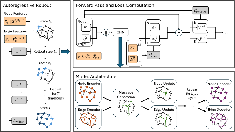
Residual connections are added at each node and edge update to stabilize predictions. From a hydrological perspective, these update operations are physically meaningful, as messages mji symbolize flow between regions and their sum Σj∈N(i)mji for node i would represent the net water flux in that region.
Decoder. After the processor block, the final embedding matrices of the nodes and edges, HL and ϵL, are translated back to the prediction feature space through a decoder, generating the final output of the model. Similar to the encoder, two separate modules are used to produce predictions for each type of structure. This decoding operation can be summarized by Eqs. 9 & 10 as
where ∆V t+1 = R|V| and ∆⃗Qt+1 = R|E| are the respective node and edge predictions.
Learnable Parameters. The encoders, decoders and message passing functions are all implemented as MLPs with LMLP layers. A ReLU activation function is added after each layer l except for the final layer LMLP -1. This is mathematically expressed in Eqs. 11 & 12:
where x are the processed embeddings and W is a matrix with learnable parameters. Following the design of SWEGNN [Bentivoglio et al., 2023], the bias term is omitted to prevent spurious water volume predictions in isolated nodes distant from the flood extent, a modification empirically demonstrated to improve flood classification.
4.2 Physics-Informed Loss Function
Multi-task Prediction Loss. The base training objective is formulated as a multi-task loss consisting of the mean squared error of node and edge predictions, as defined in Eqs. 13 & 14.
The total prediction loss can then be computed as a weighted sum between these two terms, expressed in Eq. 15:
where the coefficients λ1 and λ2 dictate the contribution of Lnode and Ledge in Lpred.
Mass Balance Regularization. To ground model predictions in physical realism, we utilize additional regularization terms derived from the conservation of mass from the Shallow Water Equations, the fundamental principles governing 2D flood movement [Costabile et al., 2017]. If assuming constant density, mass conservation is equivalent to volume conservation, enabling formulation using volumetric quantities aligned with the model's predictions. Given a control volume CV , this can be expressed as
where ⃗Q+ and ⃗Q- is the influx and efflux through CV , and ⃗Qsources and ⃗Qsinks are flows adding and removing water from the system. The physics-informed loss is comprised of global mass loss Lglobal and local mass loss Llocal, which is written in Eq. 17 as
where the coefficients λ3 and λ4 balance the contribution of Lglobal and Llocal in Lphysics. We now explain the formulation of Lglobal and Llocal.
Global-level Regularization. Global mass conservation considers the entire target catchment as the control volume CV . We define the global mass conservation loss as follows (Eq. 18):
where ∆V t i = V t+1 i - V t i is the change in volume at node i from the current timestep t to the next timestep t+1 and ∆t is the temporal resolution between consecutive timesteps. The regularization term is based on the absolute value of the mass balance residual, resulting in a well-defined convex objective (Lglobal = 0) for gradient-based optimization. Notably, this form of regularization is only applied to node volume predictions V as the other variables ⃗Qin, ⃗Qout and R are given to the model as boundary conditions.
Local-level Regularization. Mass conservation was also explicitly enforced on a local scale considering each individual node i as the control volume CV . We define the local mass conservation loss as follows (Eq. 19):
where ⃗Qi+ and ⃗Qi- are the respective inflow and outflow at a node i. Taking the absolute value is performed for the same reasons previously mentioned, where Llocal = 0 corresponds to perfect conservation at all nodes. Unlike the global regularization term, this condition balances both node water volume V and edge water flow ⃗Q predictions.
The inflow ⃗Qi+ and outflow ⃗Qi- at each node are computed directly from the edge predictions ⃗Q. Given the COO adjacency matrix I, let I′ = R2×|E| be the transposed adjacency matrix such that I′ = {(j, i) | (i, j) ∈ I}. The undirected adjacency matrix Iundir = R2×2|E| can then be represented as in Eq. 20.
Weights are generated for each edge in Iundir representing the flow along its direction through Eq. 21.
where ⊙ is the element-wise product. Applying ReLU(·) removes negative values of ⃗Q, which indicate flow opposite to the edge direction, leaving only positive weights. The total inflow is then computed for each node i as in Eq. 22:
where Nin(i) are the edges pointing towards node i. Similarly, the total outflow at each node is denoted as in Eq. 23:
where Nout(i) are the edges pointing away from node i.
Overall Loss. The overall loss function is derived by taking the sum of the prediction loss and physics loss, defined in Eq. 24:
4.3 Autoregressive Training
Multi-step-ahead Loss. Multi-step predictions are obtained through autoregressive inference that introduces gradually accumulating errors. The typical supervised or teacher forcing training strategy is unable to handle such distribution shifts [Teutsch and M¨ader, 2022]. We adopt the approach of Bentivoglio et al. [2023], which proposes the use of a multistep-ahead loss to allow the model to develop robustness to its own noisy input. For each training batch, an autoregressive rollout is performed, after which the total loss used for backpropagation is calculated as in Eq. 25:
where O is the rollout length and L is the overall loss defined in Eq. 24. This procedure is particularly crucial for the application of the physics-informed loss, as during multi-step rollouts, the constrained hydrological states are given purely by the model's predictions. Thus, not only does the model learn to correct its own errors, but to do so in a manner that adheres to mass conservation throughout the trajectory.
Dynamic Curriculum Learning. To improve training stability, the original implementation utilizes a curriculum learning strategy [Bentivoglio et al., 2023]. The model is initially trained on the simpler task of predicting 1-step-ahead loss, which is gradually increased at a 1-step increment after a set number of epochs until it finally reaches the target rollout length O. However, this deterministic approach fails to accommodate the non-uniform difficulty of predicting varying time horizons. To create a more adaptive progression, this fixed schedule is replaced with an early stopping mechanism, where the prediction horizon is extended only after the model's performance has converged on the validation set for the current rollout length o. Furthermore, we design the step size between curriculum stages to be a tunable hyperparameter C, which controls the learning progression. To mitigate catastrophic interference, the learning rate is decayed by a factor γ after each curriculum step. This entire process can be interpreted as a sequence of fine-tuning steps, where a converged model for a given horizon is adapted for the subsequent, more challenging longer rollout duration.
5 Experiments
5.1 Experimental Setup
Dataset. The target catchment for this studywas taken from a section of the Wollombi River watershed located in New South Wales, Australia. A dataset comprised of 56 flowdominant flood events was generated using the HEC-RAS numerical model [Brunner, 2025]. The 2D unstructured mesh was converted to a directed graph composed of 1129 nodes and 2743 edges. Each event consists of 576 time steps with a resolution of 15 minutes.
| Model | RMSE (m3 ) ↓ | MAE (m3 ) ↓ |
|---|---|---|
| GCN (node) | 9,849.98 ± 2,485.73 | 6,340.51 ± 1,859.60 |
| GAT (node) | 13,232.86 ± 11,835.18 | 4,583.68 ± 1,969.27 |
| GraphSAGE (node) | 11,146.97 ± 11,420.79 | 4,177.75 ± 2,519.14 |
| GIN (node) | 5,023.18 ± 1,450.37 | 2,587.05 ± 798.38 |
| GINE (node) | 3,437.68 ± 693.94 | 1,860.03 ± 406.78 |
| HydroGraphNet | 7,584.51 ± 3,068.54 | 3,343.52 ± 1,392.34 |
| DUALFloodGNN | 2,216.27 ± 868.21 | 1,075.63 ± 394.83 |
Baselines. The DUALFloodGNN architecture was compared to standard GNN models such as Graph Convolutional Network (GCN) [Kipf and Welling, 2017], Graph Attention Network (GAT) [Veliˇckovi´c et al., 2018], Graph SAmple and aggreGatE (GraphSAGE) [Hamilton et al., 2018], Graph Isomorphism Network (GIN) [Xu et al., 2019], and Graph Isomorphism Network with Edges (GINE) [Hu et al., 2020]. Variations of these models for edge regression were created by incorporating an MLP prediction head that leverages the features of adjacent nodes to predict edge values. The proposed architecture was also compared to domain-specific GNN models, including HydroGraphNet [Taghizadeh et al., 2025] and SWE-GNN [Bentivoglio et al., 2023]. Models were evaluated for the water volume, flow and depth prediction tasks through 14-fold cross validation.
Metrics. Performance for the regression tasks was measured using Root Mean Squared Error (RMSE) and Mean Absolute Error (MAE) per timestep. To measure flood extent classification, Critical Success Index (CSI), which is defined in Eq. 26, was computed by classifying flooded nodes for the thresholds τ = 0.05 m and τ = 0.3 m, following the convention in other literature [Bentivoglio et al., 2023; Herath et al., 2025; Taghizadeh et al., 2025].
5.2 Experimental Results
Overall Results. The results for the water volume and flow prediction task are shown in tables 1 and 2 respectively. For node volume prediction, DUALFloodGNN yielded the best results out of all the models, surpassing the RMSE of the second best model, GINE, by 35.53%. The proposed model maintained its superior standing for edge flow regression compared to other benchmarked GNNs, improving the baseline RMSE by 41.21%. Notably, baseline models that incorporated edge attributes (GAT and GINE) performed significantly worse in flow prediction, highlighting the importance of joint node and edge modeling for utilizing edge features. In terms of variability, DUALFloodGNN exhibited stable performance across different test sets, yielding a low standard deviation. Moreover, only DUALFloodGNN obtained metrics for both water volume and flow within a single model whereas other baseline architectures required multiple models for each prediction task.
| Model | RMSE (m3 /s) ↓ | MAE (m3 /s) ↓ |
|---|---|---|
| GCN (edge) | 90.99 ± 25.04 | 40.37 ± 10.47 |
| GAT (edge) | 263.40 ± 63.16 | 60.11 ± 13.90 |
| GraphSAGE (edge) | 44.02 ± 12.54 | 17.05 ± 4.48 |
| GIN (edge) | 51.21 ± 16.33 | 22.64 ± 7.61 |
| GINE (edge) | 249.31 ± 70.59 | 58.38 ± 15.56 |
| DUALFloodGNN | 25.88 ± 9.64 | 11.40 ± 4.17 |
| Model | RMSE ↓ (m) | MAE ↓ (m) | CSI ↑ | Inference Time (s) | |
|---|---|---|---|---|---|
| τ = 0.05m | τ = 0.3m | ||||
| HydroGraphNet | 0.76 ±0.34 | 0.29 ±0.16 | 0.69 ±0.13 | 0.80 ±0.05 | 3.25 ±0.17 |
| SWE-GNN | 1.23 ±0.35 | 0.61 ±0.21 | 0.47 ±0.11 | 0.49 ±0.09 | 7.21 ±0.20 |
| DUALFloodGNN | 0.21 ±0.07 | 0.07 ±0.03 | 0.90 ±0.03 | 0.91 ±0.03 | 4.10 ±0.06 |
Each flood GNN model's performance was evaluated for water depth prediction given its prevalence in practical usecases. Water depth was back calculated from DUALFloodGNN's predictions with a volume-to-elevation mapping provided in the HEC-RAS simulation. As observed in table 3, the proposed model continued to outperform even domainspecific models, yielding a 72.37% improvement to the second best RMSE. In terms of classification, DUALFloodGNN accurately categorized flooded nodes by achieving a similar CSI of around 0.9 in both 0.05 and 0.3 m thresholds. SWE-GNN showed the same trend albeit at a much lower accuracy, while HydroGraphNet displayed a high delta between its CSI for the two cases. With regards to inference speed, DUALFloodGNN closely matches the low latency of HydroGraphNet with only a 0.85 second difference. Thus, DUALFLoodGNN preserves the same 2 to 3 orders of magnitude speed-up compared to numerical solvers as reported by the previous studies [Bentivoglio et al., 2023; Taghizadeh et al., 2025]. For example, an event that would take almost a day to run for a numerical model would only take around 3 minutes for our model to simulate.
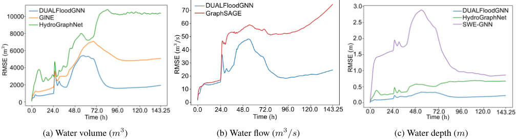
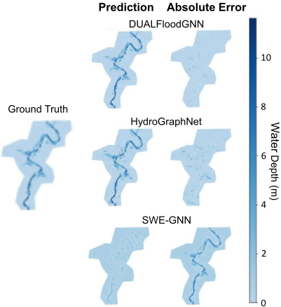
Event Analysis. The water volume, flow and depth RMSE per timestep of select GNNs were plotted for a single case study event in figure 3. Across all tasks, DUALFloodGNN exhibited superior temporal stability, consistently maintaining the lowest RMSE values throughout the entire rollout period. To visualize flood extent, max flood depth maps, which plot the maximum water depth for each node in the graph across all timesteps, were generated for the selected event (figure 4). In the ground truth, the nodes with the highest water depth are located near the river area where flow is most concentrated. SWE-GNN predicted mostly uniform flood propagation throughout the catchment while HydroGraphNet overestimated flooding for a few nodes far from the central river area. DUALFloodGNN produced the most accurate map, demonstrating its capacity to capture the flood's
0
Figure 4: Maximum water depth map of flood-specific GNN models for the case study event. The maps of the ground truth, model predictions (left) and difference between the two (right) are shown.
microscale dynamics.
5.3 Ablation Studies
Table 4 summarizes the ablation studies performed to identify the key factors contributing to the model's performance.
Global Inflow Feature. The exclusion of the global inflow Qin significantly affected the predictive accuracy of the model. The inclusion of this global feature [Battaglia et al., 2018] for all nodes is an approach directly adopted from HydroGraphNet [Taghizadeh et al., 2025], which demonstrated the same degradation in performance when omitted. This could be attributed to the flow-dominant nature of the flood events in the dataset. We enhanced the global inflow feature by treating it as a dynamic feature, also including the previous boundary conditions as model input.
Physics-informed Loss Three additional physics-informed variants were considered: only global loss, only local loss and no physics-informed loss. In contrast to applying only global mass balance, integrating local-level regularization resulted in a lower RMSE for both node and edge prediction, surpassing the accuracy of the purely data-driven model. This can be attributed to the co-dependent modeling of node and edge outputs in the local physics loss. A model with physics constraints on both scales demonstrates comparable overall performance to one with only local loss, though the superior variant varies across testing folds. Thus, selection between the two should be driven by empirical evaluation on the target dataset.
| Model | Node RMSE ↓ (m3 ) | Edge RMSE ↓ (m3 /s) |
|---|---|---|
| DUALFloodGNN | 2,216.27 ± 868.21 | 25.88 ± 9.64 |
| No Inflow Feature | 20,562.71 ± 8,054.11 | 423.40 ± 246.11 |
| Global Loss Only | 2,794.10 ± 851.61 | 48.09 ± 14.52 |
| Local Loss Only | 2,116.45 ± 845.44 | 26.07 ± 8.55 |
| No Physics Loss | 2,640.42 ± 1011.80 | 46.86 ± 15.81 |
| HydroGraphNet | 7,584.51 ± 3,068.54 | - |
| No Inflow Feature | 20,867.39 ± 6697.08 | - |
6 Conclusion
In conclusion, this study presents DUALFloodGNN, a novel physics-informed flood GNN, that explicitly incorporates global and local mass conservation within the loss function. To this end, it performs simultaneous node and edge prediction, jointly modeling these values through a shared message passing operation. To enhance robustness, the model is trained with a dynamic curriculum learning strategy, which adjusts the learning period in response to the current difficulty. DUALFloodGNN outperformed standard GNN architectures and state-of-the-art GNN flood models in the prediction of hydrodynamic variables and the classification of flooded locations. Additionally, the model maintained computational efficiency comparable to other flood-specific GNN approaches, demonstrating its suitability for operational use cases.
Future research can evaluate the model's generalizability for other catchments and flood types. For example, in flows with high sediment or debris concentration, density is not spatially uniform which may affect volume-based regularization.
@inproceedings{ijcai2026p713,
  title     = {DUALFloodGNN: Physics-informed Graph Neural Network for Operational Flood Modeling},
  author    = {Acosta, Carlo Malapad and Herath, Herath Mudiyanselage Viraj Vidura and Lim, Jia Yu and Saha, Abhishek and Rasnayaka, Sanka and Marshall, Lucy},
  booktitle = {Proceedings of the Thirty-Fifth International Joint Conference on
               Artificial Intelligence, {IJCAI-26}},
  publisher = {International Joint Conferences on Artificial Intelligence Organization},
  editor    = {Diego Calvanese},
  pages     = {6408--6416},
  year      = {2026},
  month     = {8},
  note      = {AI4Tech: AI Enabling Technologies},
  doi       = {10.24963/ijcai.2026/713},
  url       = {https://doi.org/10.24963/ijcai.2026/713},
}
TY - CPAPER TI - DUALFloodGNN: Physics-informed Graph Neural Network for Operational Flood Modeling AU - Acosta, Carlo Malapad AU - Herath, Herath Mudiyanselage Viraj Vidura AU - Lim, Jia Yu AU - Saha, Abhishek AU - Rasnayaka, Sanka AU - Marshall, Lucy T2 - Proceedings of the Thirty-Fifth International Joint Conference on Artificial Intelligence, IJCAI-26 PB - International Joint Conferences on Artificial Intelligence Organization PY - 2026 SP - 6408 EP - 6416 DO - 10.24963/ijcai.2026/713 UR - https://doi.org/10.24963/ijcai.2026/713 ER -Copied
Machine-readable versions of this paper, for tools and AI agents:





