
Mining Statistically Likely k-Reachable States in Probabilistic Programs
Proceedings of the Thirty-Fifth International Joint Conference on Artificial Intelligence. Main Track. Pages 6398-6406.
https://doi.org/10.24963/ijcai.2026/712
Keywords
- Uncertainty in AI: Probabilistic programming
Abstract
We propose the notion of statistically likely k-step reachable set in probabilistic programs, a statistically robust notion for high-probability k-step reachable program states. We design an inductive algorithm to capture this set as a symbolic representation in propositional logic for Boolean probabilistic programs. Our methodology iteratively learns a symbolic formula for the statistically likely k-step reachable set that involves (a) learning an initial symbolic candidate via decision tree learning, (b) collecting positive and negative counterexamples via forward and backward verification checks, and (c) refining the current candidate via a sequence of prune and split moves on the decision tree. We demonstrate that the statistically likely k-step reachable set can reveal interesting properties about programs by studying probabilistic programs from the literature.
- [Aiken et al., 2016] Andrew Aiken, Marco Corradini, and Daniel Strubell. From Invariant Checking to Invariant In- ference Using Randomized Search. In Proceedings of the 28th International Conference on Computer Aided Verifi- cation (CAV), pages 388-402, 2016.
- [Bao et al., 2024] Jialu Bao, Nitesh Trivedi, Drashti Pathak, Justin Hsu, and Subhajit Roy. Data-driven invariant learn- ing for probabilistic programs. Formal Methods in System Design, 66:278-306, 2024.
- [Bartocci et al., 2020] Ezio Bartocci, Laura Kovács, and Miroslav Stankovič. Mora: Automatic Generation of Moment-Based Invariants. In Proceedings of the 26th In- ternational Conference on Tools and Algorithms for the Construction and Analysis of Systems (TACAS), pages 492-498, 2020.
- [Batz et al., 2023] Kevin Batz, Mingshuai Chen, Sebastian Junges, Benjamin Lucien Kaminski, Joost-Pieter Katoen, and Christoph Matheja. Probabilistic Program Verifica- tion via Inductive Synthesis of Inductive Invariants. In Proceedings of the 29th International Conference on Tools and Algorithms for the Construction and Analysis of Sys- tems (TACAS), pages 410-429, 2023.
- [Biere et al., 1999] Armin Biere, Alessandro Cimatti, Ed- mund M. Clarke, and Yunshan Zhu. Symbolic model checking without BDDs. In Proceedings of the 5th Inter- national Conference on Tools and Algorithms for the Con- struction and Analysis of Systems (TACAS), pages 193- 207, 1999.
- [Biere et al., 2024] Armin Biere, Tobias Faller, Katalin Fazekas, Mathias Fleury, Nils Froleyks, and Florian Pol- litt. CaDiCaL 2.0. In Proceedings of the 36th International Conference on Computer Aided Verification (CAV), pages 133-152, 2024.
- [Chakraborty et al., 2023] Saikat Chakraborty, Shuvendu Lahiri, Sarah Fakhoury, Akash Lal, Madanlal Musuvathi, Aseem Rastogi, Aditya Senthilnathan, Rahul Sharma, and Nikhil Swamy. Ranking LLM-Generated Loop Invariants for Program Verification. In Proceedings of the 2023 Con- ference on Empirical Methods in Natural Language Pro- cessing (EMNLP), pages 9164-9175, 2023.
- [Chen et al., 2015] Yu-Fang Chen, Chih-Duo Hong, Bow- Yaw Wang, and Lijun Zhang. Counterexample-Guided Polynomial Loop Invariant Generation by Lagrange Inter- polation. In Proceedings of the 27th International Confer- ence on Computer Aided Verification (CAV), pages 658- 674, 2015.
- [Das and Lal, 2017] Ankush Das and Akash Lal. Precise null pointer analysis through global value numbering. In Pro- ceedings of the 15th International Symposium on Auto- mated Technology for Verification and Analysis (ATVA), pages 25-41, 2017.
- [Das et al., 2015] Ankush Das, Shuvendu K. Lahiri, Akash Lal, and Yi Li. Angelic Verification: Precise Verification Modulo Unknowns. In Proceedings of the 27th Interna- tional Conference on Computer Aided Verification (CAV), pages 324-342, 2015.
- [Ezudheen et al., 2018] P. Ezudheen, Daniel Neider, Deepak D'Souza, Pranav Garg, and P. Madhusudan. Horn- ICE Learning for Synthesizing Invariants and Contracts. Proceedings of the ACM on Programming Languages, 2(OOPSLA):131:1-131:25, 2018.
- [Feng et al., 2017] Yijun Feng, Lijun Zhang, David N. Jansen, Naijun Zhan, and Bican Xia. Finding Polynomial Loop Invariants for Probabilistic Programs. In Proceed- ings of the 15th International Symposium on Automated Technology for Verification and Analysis (ATVA), pages 400-416, 2017.
- [Garg et al., 2014] Pranav Garg, Christof Löding, P. Mad- husudan, and Daniel Neider. ICE: A robust framework for learning invariants. In Proceedings of the 26th Interna- tional Conference on Computer Aided Verification (CAV), volume 8663 of Lecture Notes in Computer Science, pages 69-87, 2014.
- [Garg et al., 2016] Pranav Garg, Daniel Neider, P. Madhusu- dan, and Dan Roth. Learning Invariants using Decision Trees and Implication Counterexamples. In Proceedings of the 43rd Annual ACM SIGPLAN-SIGACT Symposium on Principles of Programming Languages (POPL), pages 499-512, 2016.
- [Gehr et al., 2016] Timon Gehr, Sasa Misailovic, and Martin Vechev. PSI: Exact Symbolic Inference for Probabilistic Programs. In Proceedings of the 28th International Con- ference on Computer-Aided Verification (CAV), pages 62- 83, 2016.
- [Gehr et al., 2020] Timon Gehr, Samuel Steffen, and Martin Vechev. λPSI: Exact Inference for Higher-Order Proba- bilistic Programs. In Proceedings of the 41st ACM SIG- PLAN Conference on Programming Language Design and Implementation (PLDI), pages 883-897, 2020.
- [Geldenhuys et al., 2012] Jaco Geldenhuys, Matthew B. Dwyer, and Willem Visser. Probabilistic Symbolic Execu- tion. In Proceedings of the 2012 International Symposium on Software Testing and Analysis (ISSTA), pages 166-176, 2012.
- [Golia et al., 2021] Priyanka Golia, Mate Soos, Sourav Chakraborty, and Kuldeep S. Meel. Designing Samplers is Easy: The Boon of Testers. In Proceedings of the 21st Conference on Formal Methods in Computer-Aided De- sign (FMCAD), pages 222-230, 2021.
- [Gretz et al., 2013] Friedrich Gretz, Joost-Pieter Katoen, and Annabelle McIver. Prinsys: On a Quest for Probabilistic Loop Invariants. In Proceedings of the 10th international conference on Quantitative Evaluation of Systems (QEST), pages 193-208, 2013.
- [Joshi et al., 2012] Saurabh Joshi, Shuvendu K. Lahiri, and Akash Lal. Underspecified Harnesses and Interleaved Bugs. Proceedings of the 39th annual ACM SIGPLAN- SIGACT symposium on Principles of programming lan- guages (POPL), pages 19-30, 2012.
- [Kaminski and Katoen, 2017] Benjamin Lucien Kaminski and Joost-Pieter Katoen. A Weakest Pre-Expectation Se- mantics for Mixed-Sign Expectations. In Proceedings of the 32nd Annual ACM/IEEE Symposium on Logic in Com- puter Science (LICS), pages 1-12, 2017.
- [Kozen, 1977] Dexter Kozen. Lower Bounds for Natural Proof Systems. In Proceedings of the 18th Annual Sympo- sium on Foundations of Computer Science (FOCS), pages 254-266, 1977.
- [Kwiatkowska et al., 2011] Marta Kwiatkowska, Gethin Norman, and David Parker. PRISM 4.0: Verification of Probabilistic Real-Time Systems . In Proceedings of the 23rd International Conference on Computer Aided Verification (CAV), pages 585-591, 2011.
- [Lahiri and Roy, 2022] Sumit Lahiri and Subhajit Roy. Al- most Correct Invariants: Synthesizing Inductive Invariants by Fuzzing Proofs. In Proceedings of the 31st ACM SIG- SOFT International Symposium on Software Testing and Analysis (ISSTA), pages 352-364, 2022.
- [Moura and Bjørner, 2008] Leonardo De Moura and Niko- laj Bjørner. Z3: An Efficient SMT Solver. In Proceed- ings of the 14th International Conference on Tools and Algorithms for the Construction and Analysis of Systems (TACAS), pages 337-340, 2008.
- [Ray et al., 2026] Arnab Ray, Nitesh Trivedi, Ansuman Banerjee, Sourav Chakraborty, Arijit Ghosh, and Subha- jit Roy. Mining Statistically Likely k-Reachable States in Probabilistic Programs, 2026. An extended abstract of this paper will appear in IJCAI 2026. Full version available at https://github.com/arnab-007/PRORP . [Riley and Fedyukovich, 2022] Daniel Riley and Grigory Fedyukovich. Multi-Phase Invariant Synthesis. In Pro- ceedings of the 30th ACM Joint European Software Engi- neering Conference and Symposium on the Foundations of Software Engineering (ESEC/FSE), pages 607-619, 2022. Link
- [Ryan et al., 2019] Gabriel Ryan, Justin Wong, Jianan Yao, Ronghui Gu, and Suman Jana. Cln2inv: learning loop in- variants with continuous logic networks. arXiv preprint arXiv:1909.11542, 2019.
- [Sharma et al., 2013] Rahul Sharma, Saurabh Gupta, Bharath Hariharan, Alex Aiken, and Aditya V. Nori. Veri- fication as Learning Geometric Concepts. In Proceedings of the 20th International Symposium on Static Analysis (SAS), volume 7935 of Lecture Notes in Computer Science, pages 388-411, 2013.
- [Si et al., 2018] Xujie Si, Hanjun Dai, Mukund Raghothaman, Mayur Naik, and Le Song. Learning Loop Invariants for Program Verification. In Proceedings of the 32nd International Conference on Neural Informa- tion Processing Systems (NeurIPS), pages 7762-7773, 2018.
- [Soos et al., 2023] Mate Soos, Divesh Aggarwal, Sourav Chakraborty, Kuldeep S. Meel, and Maciej Obremski. En- gineering an Efficient Approximate DNF-counter. In Pro- ceedings of the 32nd International Joint Conference on Ar- tificial Intelligence (IJCAI), pages 2031-2038, 2023. IJCAI
- [Susag et al., 2022] Zachary Susag, Sumit Lahiri, Justin Hsu, and Subhajit Roy. Symbolic execution for random- ized programs. Proceedings of the ACM on Programming Languages 2, 6(OOPSLA):1583-1612, 2022.
- [Wang et al., 2018] Di Wang, Jan Hoffmann, and Thomas Reps. PMAF: An Algebraic Framework for Static Anal- ysis of Probabilistic Programs. Proceedings of the 39th ACM SIGPLAN Conference on Programming Language Design and Implementatio (PLDI), pages 513-528, 2018.
- [Wu et al., 2024] Guangyuan Wu, Weining Cao, Yuan Yao, Hengfeng Wei, Taolue Chen, and Xiaoxing Ma. LLM Meets Bounded Model Checking: Neuro-Symbolic Loop Invariant Inference. In Proceedings of the 39th IEEE/ACM International Conference on Automated Software Engi- neering (ASE), pages 406-417, 2024.
- [Yao et al., 2020] Jianan Yao, Gabriel Ryan, Justin Wong, Suman Jana, and Ronghui Gu. Learning Nonlinear Loop Invariants with Gated Continuous Logic Networks. In Pro- ceedings of the 41st ACM SIGPLAN International Confer- ence on Programming Language Design and Implementa- tion (PLDI), pages 106-120, 2020.
- [Yu et al., 2023] Shiwen Yu, Ting Wang, and Ji Wang. Loop Invariant Inference through SMT Solving Enhanced Re- inforcement Learning. In Proceedings of the 32nd ACM SIGSOFT International Symposium on Software Testing and Analysis (ISSTA), pages 175-187, 2023.
References were extracted automatically from the PDF and may contain errors.
Full text extracted automatically from the PDF; figures, tables and equations may differ. The PDF is the version of record.
1 Introduction
Symbolic analysis has significantly advanced the state-of-theart for program verification. Such analyzers compute a symbolic representation of a target program, commonly in some fragment of logic, and use satisfiability engines (SAT solvers) to search for proofs and counterexamples. However, verification of real-world programs remains challenging. The primary difficulty is the challenge in modeling the uncertainties presented by the environment within which a program is executing. The environment can, though sparingly, provide unexpected values that deviate the program from its "regular" set of reachable states. For example, a memory allocation using a malloc() may infrequently fail (return NULL), that may require executing an exception handling routine.
A possible strategy is to model the environment as a stochastic process, where the probability distribution over different kinds of failures can be based on recommendation of domain experts or estimated from empirical studies. This allows us to ignore rare events and understand the commoncase behaviors of the program. We refer to such a set of reachable states as statistically likely k-step reachable set.
∗ For full version of the paper and the artifact, see https://github. com/arnab-007/PRORP
In this work, we attempt to synthesize the statistically likely k-step reachable set for such probabilistic programs. Such reachable sets have applications in program understanding as the computed reachable sets do not include corner-case exception states. Further, along the lines of prior work like angelic verification [Das et al., 2015; Das and Lal, 2017; Joshi et al., 2012; Lahiri and Roy, 2022], the attempt to identify potential false positives that are signaled due to unduly demonic assumptions about the environment, statistically likely k-step reachable set can also have applications in sieving through false positives for real bugs. Our approach uses a combination of formal and learning based approaches to tackle this problem. Symbolically characterizing the common-case behaviors of probabilistic programs is a core problem in AI, with applications spanning Bayesian inference, AI safety, and bug prioritization. We address this by learning a symbolic posterior summary that distinguishes high-probability program behaviors from rare corner cases.
Contributions
The contributions of this work are as follows:
- We propose the notion of statistically likely k-step reachable set ϵ-Clk(φ), a symbolic characterization of states that probabilistic programs reach with nonnegligible probability;
- We prove that even the problem of deciding the emptiness of ϵ-Clk(φ) is itself computationally hard, which motivates approximate solutions;
- We design an algorithm to compute this set with statistical guarantees, which to our knowledge is the first framework to learn symbolic approximation of highprobability reachable sets;
- We build our algorithm into a tool, PRORP, and use it to study the statistically likely k-step reachable set on probabilistic programs from literature.
2 Preliminaries
2.1 Boolean Formulas, Satisfiability and Samplers
For a Boolean formula φ, we use Supp(φ) to denote the set of variables appearing in φ. An assignment σ ∈ {0, 1}|Supp(φ)| to Supp(φ) is a satisfying assignment or witness if it makes φ
evaluate to 1. We denote the set of all satisfying assignments of φ as Rφ and say a formula φ represents the set Rφ.
A formula is in conjunctive normal form (CNF) (resp. disjunctive normal form (DNF)) if it is a conjunction (resp. disjunction) of one or more clauses (resp. terms), where each clause (resp. term) is a disjunction (resp. conjunction) of literals. A literal is a variable or its negation.
Definition 1 (Uniform samplers). A uniform-CNF-sampler (resp. uniform-DNF-sampler) is a randomized algorithm A that takes as input a CNF-formula (resp. DNF-formula) φ and outputs a satisfying assignment of φ uniformly at random from the set of all satisfying assignments. That is, for any σ ∈ Rφ, Pr[A outputs σ] = 1 |Rφ| , where the probability is over the internal randomness used in A.
For a CNF or DNF formula φ, by drawing m iid samples from D(Rφ) we mean using the relevant samplers to draw m independent and identically distributed samples from the distribution D over the set Rφ.
2.2 Probabilistic Programs and k-Step Reachability
Definition 2 (Probabilistic programs). A probabilistic program is a tuple (X , loc, trans) where (i) X = {x1, . . . , xn} is a finite set of Boolean program variables, (ii) loc is a finite set of control locations and (iii) trans is a finite set of transitions, each of the form (ℓ, guard) ⇒ {(p1, u1, ℓ′1 ), . . . , (pm, um, ℓ′m)}, where ℓ, ℓ′i ∈ loc, ∑i pi = 1, each ui is a deterministic update over X, and when the Boolean predicate guard holds at ℓ, the program moves to ℓ′i applying ui with probability pi.
Programs defined over variables taking values in a bounded integer domain can be encoded as a finite propositional formula via bit-blasting, a technique formalized in [Biere et al., 1999]. The encoding extends naturally to probabilistic programs over finite domains [Kwiatkowska et al., 2011].
Definition 3 (Program states). Given a probabilistic program P defined over a set of Boolean program variables X , a program state σ is a mapping from X to {0, 1}|X| , i.e., it is a valuation over the program variables. Thus, the entire program state space can be represented as ΩP := {0, 1}|X| .
Example: Consider a boolean probabilistic program P defined over a non-negative integer variable z and a Boolean flag flip. For 3-bit encoding of z = z2z1z0 with X = {z2, z1, z0, flip}, the state space is given by ΩP = {0, 1}4 . An example of a program state is {z2 = z0 = 1, z1 = 0, flip = 0} which corresponds to (z = 5, flip = 0).
Definition 4 (k-step transition and terminal states). For a probabilistic program P defined over program variables X with ΩP being the entire state space and for any k ∈ N, the k-step program transition probability function is a function ΓkP : ΩP ×ΩP → [0, 1] such that ΓkP (σ, σ′ ) gives the probability of reaching state σ′ from the state σ in exactly k steps. So clearly, for all σ ∈ ΩP , ∑σ′ ΓkP (σ, σ′ ) = 1.
Let P be a probabilistic program over program variables X, and let ΩP denote its state space. A state σ ∈ ΩP is called a terminal state or sink state of P if no further program transitions are possible from σ, that is,
We denote the set of all terminal states of P by TP ⊆ ΩP . Specifically, terminal states correspond to program configurations in which the program execution has halted.
Given σ′ ∈ TP , Γ≤k P (σ, σ′ ) denotes the probability of reaching σ′ starting from σ in at most k steps, that is, Γ≤k P (σ, σ′ ) := ΓiP (σ, σ′ ), where i = min{j ∈ [1, k] | ΓjP (σ, σ′ ) > 0}, otherwise 0.
The k-step program formula F k P is a Boolean formula over 2|X | number of variables representing a k-step single execution path of the program. In other words, or any σ, σ′ ∈ ΩP , F k P (σ, σ′ ) = 1 if ΓkP (σ, σ′ ) > 0
Definition 5 (Precondition). For a probabilistic program P defined over program variables X, with ΩP being the entire state space, a precondition set is a subset Rφ of ΩP describing a possible set of valuations at the beginning of P. The subset is described implicitly by the Boolean formula φ, known as the precondition.
2.3 Compiling Decision Trees to Boolean Formula
A decision tree for a Boolean function f : {0, 1}n → {0, 1} is a rooted binary tree whose internal nodes are labeled by variables xi ∈ {x1, . . . , xn}, whose outgoing edges are labeled by the Boolean outcomes 0 and 1, and whose leaves are labeled by output values of f . Each root-to-leaf path encodes a conjunction of literals specifying an input x ∈ {0, 1}n , and the label of the leaf is the value f(x). Equivalently, a decision tree represents the function f as the disjunction of the conjunctions of the decisions along all root-to-leaf paths labeled 1 at the leaves.
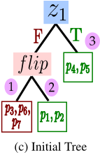
For example, the tree in Figure 1c corresponds to the DNF (z1 ∨ (¬z1 ∧ flip)). For a given decision tree T, we assume that ExtractLeaves(T) returns the list of all leaves in T, and TreeDNF(T) outputs the DNF represented by T.
3 Statistically Likely k-Step Reachable Set
To formalize the notion of statistically likely k-step reachable set, we first define the concept of k-step reachability.
Definition 6 ((At most k)-step reachability). For a precondition φ of a probabilistic program P, a k-step reachable formula with respect to precondition φ is a Boolean formula ζ that satisfies the following condition: σ′ ∈ Rζ ⇐⇒ ∃σ ∈ Rφ with (∨ki=0 F iP (σ, σ′ )) = 1. Thus, Rζ is the set of all terminal states that reachable in atmost k steps if the program P is executed with a starting state in Rφ. We call this set the k-step reachable set and denote it by Clk(φ).
Definition 7 (Atmost k-step transition probability). For a precondition φ consider the k-step reachable set Clk(φ). Then for any σ′ ∈ Clk(φ) and any given probability distribution D over the set Rφ, we define the at most k-step program transition function w.r.t. to precondition φ as ΓP,φ(σ′ ) := Eσ∼D(Rφ) [Γ≤k P (σ, σ′ )]. This quantity gives the probability of reaching the terminal state σ′ in atmost k steps from an initial state σ ∈ Rφ chosen according to D.
However, Clk(φ) is the set of all reachable states when P starts from Rφ. To only capture the states reached with "nonnegligible" probability, we introduce the concept of statistically likely k-step reachable set.
Definition 8 (Statistically likely k-step reachable set). For a probabilistic program P, a precondition φ and a threshold ϵ ∈ (0, 1], we consider the set ϵ-Clk(φ) ⊆ Clk(φ), which we call the ϵ-statistically likely k-step reachable set for P w.r.t. the precondition φ and is defined as ϵ-Clk(φ) := Clk(φ) ∩ {σ′ | ΓP,φ(σ′ ) ≥ ϵ}.
3.1 Exact Synthesis of ϵ-Clk(φ)
Given a probabilistic Boolean program P with input variables X, a distribution D from which X is sampled, precondition φ, k ∈ N representing the number of steps, and the parameter ϵ ∈ (0, 1], we refer to the task of exactly synthesizing the set ϵ-Clk(φ) as ϵ-Clk(φ) SYNTHESIS. We analyze the ϵ-Clk(φ) EMPTINESS problem (asking whether ϵ-Clk(φ) is empty), whose hardness lower-bounds that of ϵ-Clk(φ) SYNTHESIS. We prove PSPACE-hardness of ϵ-Clk(φ) EMPTINESS by a Karp reduction from the known PSPACEcomplete problem DFA-INTERSECTION [Kozen, 1977]. We state the theorem below.
Theorem 1. ϵ-Clk(φ) EMPTINESS is PSPACE-complete. This result motivates approximate synthesis of ϵ-Clk(φ). We provide the formal proof for PSPACE-completeness of the ϵ-Clk(φ) EMPTINESS problem in the full version [Ray et al., 2026] of this paper. We now formalize the problem of approximate synthesis of ϵ-Clk(φ).
3.2 Approximate Synthesis of ϵ-Clk(φ)
For a probabilistic program P and a precondition φ, a set S ⊆ Clk(φ) is called a ϵ-approximate k-step reachable set if ∑σ∈Clk(φ)\S ΓP,φ(σ) ≤ ϵ. A formula ψ representing an ϵ-approximate k-step reachable set Rψ is called an ϵapproximate k-step reachable formula. Note that, if S is any ϵ-approximate k-step reachable set, ϵ-Clk(φ) ⊆ S. Trivially, the entire state space is an ϵ-approximate k-step reachable set. So our goal is to learn an ϵ-approximate k-step reachable formula ψ whose set Rψ is close to ϵ-Clk(φ). To quantify closeness, we define two error measures between ψ and Clk(φ).
Definition 9 (Error distances for candidate formula). Given a probabilistic program P , a precondition φ and a distribution D over Rφ, the Fo-errors and Ba-errors between a candidate Boolean formula ψ and the k-step reachable set Clk(φ) are quantified as follows
- The Fo-error distance ErrorFo(ψ, Clk(φ)) is the probability that the terminal state reached after execution of atmost k steps of P on an initial state randomly picked from Rφ according to D is not satisfied by ψ. It is defined as ErrorFo(ψ, Clk(φ)) := ∑σ∈(Clk(φ)\Rψ) ΓP,φ(σ).
- The Ba-error distance ErrorBa(ψ, Clk(φ)) is a measure of the fraction of program states in Rψ that are not satisfied by Clk(φ). It is defined as ErrorBa(ψ, Clk(φ)) := Prσ∼URψ [σ ̸∈ Clk(φ)]
| φ | Rφ | ψ |
|---|---|---|
| z14 | ⋃1j=0 [(2j+1)214 , (j+1)215-1] | z14 |
| z12 | ⋃7j=0 [(2j+1)212 , (j+1)213-1] | z12 |
| z10 | ⋃31 j=0 [(2j+1)210 , (j+1)211-1] | z10 |
| z8 | ⋃127 j=0 [(2j+1)28 , (j+1)29-1] | z8∨(¯ z7∧¯ z6∧¯ z8) |
| z6 | ⋃511 j=0 [(2j+1)26 , (j+1)27-1] | True |
Definition 10 ((ϵ1, ϵ2)-approximate statistically likely k-step reachability). For any probabilistic program P , precondition φ, input distribution D over Rφ, k ∈ N and any 0 ≤ ϵ1, ϵ2 ≤ 1, a formula ψ is called a (ϵ1, ϵ2)-approximate statistically likely k-step reachable formula of P with respect to φ if ErrorFo(ψ, Clk(φ)) < ϵ1 and ErrorBa(ψ, Clk(φ)) < ϵ2.
Given P, precondition φ, 0 ≤ ϵ1, ϵ2, δ ≤ 1, and k ∈ N an algorithm is said to synthesize an (ϵ1, ϵ2, δ)-approximate statistically likely k-step reachable set of P with respect to φ if it outputs a Boolean formula ψ such that with probability at least (1 - δ), Rψ is a (ϵ1, ϵ2)-approximate statistically likely k-step reachable formula of P with respect to φ.
Let us define the problem of approximating ϵ-Clk(φ).
Problem statement: Given a probabilistic Boolean program P with input variables X , precondition φ, input distribution D over Rφ, k ∈ N representing the number of steps, and error-bounds ϵ1, ϵ2, δ ∈ (0, 1], we want to synthesize an (ϵ1, ϵ2, δ)-approximate statistically likely k-step reachable set of the probabilistic program P with respect to φ.
Clearly, for the given problem setup, the set ϵ1-Clk(φ) ⊆ S, where S is some (ϵ1, ϵ2, δ)-approximate statistically likely k-step reachable set of P with respect to φ. To solve the above problem, we introduce an algorithm PRORP. We now study the output of PRORP using an illustrative example.
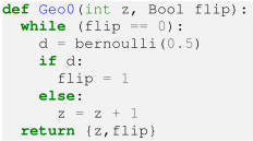
Illustrative Example. We illustrate the notion of approximate statistically likely k-step reachable set using the probabilistic program Geo0 (Figure 1a). Starting from z = 0, the program returns geometrically distributed values, so small outputs are exponentially more likely than large ones, creating a structural asymmetryhigh-order bits rarely change whereas low-order bits vary often. For a precondition ϕ, let Rϕ denote the initial states, and let ϵ-Clk(φ) be the states reachable within k iterations with probability at least ϵ. For Geo0, while Clk(φ) contains many low-probability states, ϵClk(φ) remains small and captures the common-case behavior. The results (z being a 16-bit unsigned integer) in Table 1 show that PRORP closely tracks ϵ-Clk(φ). For preconditions involving higher-order bits (z14, z12, z10), the learned candidate exactly characterizes the likely reachable states. As the precondition moves to lower-order bits, chances of leaving the initial region increases, so the formulas admit more states. In the extreme case z6, almost the entire state space becomes likely reachable, and PRORP returns True. These observations highlight the common-case behaviour of Geo0.
4 Algorithm
We use an iterative refinement strategy which "guesses" a potential candidate, and then, our verification subroutines validate the solution. Any counterexample augment the dataset and the process is repeated till a candidate is verified.
4.1 The Verification Subroutines
A candidate formula ψ for the (ϵ1, ϵ2, δ)-statistically likely kstep reachable set problem can have errors in two directions:
- The formula ψ excludes program states reachable from the inputs; we call such examples Fo-counterexamples.
- The formula ψ includes program states not reachable from the inputs; such examples are Ba-counterexamples.
We design two verification subroutines, FoRT (ForwardReachability-Tester) to test for Fo-errors and BaRT (Backward-Reachability-Tester) to test for Ba-errors. Our algorithm alternates between these two subroutines to obtain the two types of counterexamples.
FoRT
This subroutine (Algorithm 1) takes as input a probabilistic program P, a precondition φ (in CNF), an input distribution D over Rφ, a candidate formula ψ (in DNF), a closeness parameter ϵ, a confidence parameter δ and the number of steps k. It returns an estimate Error1 of the Fo-error and a multiset CEFo of Fo-counterexamples. To capture "high-probability" counterexamples, FoRT samples a set U of initial states from D(Rφ) (Line 2), executes P for at most k steps (represented by P ≤k (u) for u ∈ U in Line 5), and records the reached terminal states y1, . . . , ym (possibly with repetitions). Each violating yi is added to CEFo as a Fo-counterexample (Line 7); Error1 is the fraction of samples failing ψ (Line 8).
Sample size m is chosen so that, with probability at least (1 - δ), Error1 is a ϵ-additive approximation of the true Foerror. FoRT only requires a black-box sampling access to D.
BaRT
This subroutine (Algorithm 2) takes as input a probabilistic program P, a precondition φ (in CNF), a candidate formula ψ (in DNF), a closeness parameter ϵ, a confidence parameter δ and the number of steps k. It returns an estimate Error2 of the Ba-error and a multiset CEBa of Bacounterexamples. Recall that Ba-counterexamples are states in (Rψ \ Clk(φ)), and true Ba-error is |Rψ\Clk(φ)| |Rψ | . To generate Ba-counterexamples, BaRT samples m states from Rψ using a uniform-like DNF-sampler (Line 2) and checks if the samples are in Clk(φ) via a SAT-solver (Line 6). The formula Υi (in line 5) encodes "is the sampled state v in Clk(φ)." If v is not in Clk(φ) then it is a Ba-counterexample and is added to the multi-set CEBa (in line 7) and the Error2 (updated in line 8) records what fraction of the samples that are drawn fromRψ are not is Clk(φ). Since our objective is to track the unreachable states in Rψ, we give equal importance to these states by sampling from the uniform distribution U over Rψ.
We choose sample size m so that with probability at least (1-δ), Error2 is a ϵ-additive approximation of true Ba-error.
Algorithm 1 FoRT (P, φ, D, ψ, ϵ, δ, k)
1: m← ⌈ 2 ϵ2 log 4δ ⌉ 2: U ←m iid samples fromD(Rφ) 3: CEFo ← ∅, Error1 ← 0 4: for u ∈ U do 5: y ← P ≤k (u) 6: if y /∈ Rψ then 7: CEFo ← CEFo ∪ {y} 8: Error1 ← Error1 + 1m- 9: return (Error1, CEFo)
Algorithm 2 BaRT(P, φ, ψ, ϵ, δ, k)
1: m← ⌈ 2 ϵ2 log 4δ ⌉ 2: V ←m iid samples from U(Rψ) 3: CEBa ← ∅, Error2 ← 0 4: for v ∈ V do 5: Υ←φ(X0) ∧ ∧j<k FP (Xj,Xj+1) ∧ ∨j≤k (Xj = v) 6: if Υ is UNSAT then 7: CEBa ← CEBa ∪ {v} 8: Error2 ← Error2 + 1m- 9: return (Error2, CEBa)
4.2 The Refinement Subroutine
TreeRepair (Algorithm 3) repairs the decision-tree representation of a candidate formula ψ using Fo and Ba counterexamples. It takes as input a decision tree T, counterexample sets CEFo and CEBa, thresholds Th1, Th2, and the variable set X . It aims to modify T so that no more than Th1 members of CEFo and Th2 members of CEBa remain misclassified.
The algorithm operates in rounds. At each round it first identifies the set L of current leaves using ExtractLeaves (line 4) and considers every potential refinement (ℓ, µ) ∈ L× ({Prune} ∪ ({Split} × X)). Each refinement is one of:
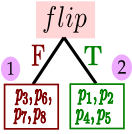
- Prune: delete a leaf node ℓ and then reclassifying all states assigned to that subtree. E.g., pruning node id 3 reduces both Error1 and Error2 to 0 (Figure 1e). The cost of the prune operation is 1.
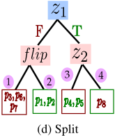
- Split: replace a leaf ℓ with an internal decision on some variable in X, creating two new leaves. For example, splitting node id 3 on predicate flip also eliminates all errors (Figure 1d). Splitting incurs cost 2.
For each potential refinement (ℓ, µ), GetGain (line 6) computes the number of counterexamples that would be correctly classified if the refinement were applied, and GetCost (line 7) returns the "cost" for making the refinement corresponding to (ℓ, µ). Finally, in line 8, a ratio Impact(ℓ,µ) of the gain to cost is calculated for each potential refinement. A refinement is sampled randomly with probability proportional to Impact (line 9) and applied via MakeTheMove (line 10). The set of counterexamples is appropriately refined by removing those that have already been addressed. Refinements occur in a top-down manner: shallow splits result in coarse approximations of the reachable region, whereas deeper splits
Algorithm 3 TreeRepair(Tinit, CEFo, CEBa, Th1, Th2, X )
- 1: Initialize T←Tinit 2: Initialize E1 ← CEFo, E2 ← CEBa 3: while NOT (|E1| ≤ Th1 and |E2| ≤ Th2) do 4: L← ExtractLeaves(T) 5: for (ℓ, µ) ∈ L × ({Prune} ∪ ({Split} × X )) do 6: Gain(ℓ,µ) ← GetGain(T, E1, E2, ℓ, µ) 7: Cost(ℓ,µ) ← GetCost(T, E1, E2, ℓ, µ) 8: Impact(ℓ,µ) ← Gain(ℓ,µ) Cost(ℓ,µ) 9: Sample (ℓ, µ) with probability proportional to Impact(ℓ,µ) 10: T,E1,E2 ← MakeTheMove(T,E1,E2, ℓ, µ) 11: Output T
Algorithm 4 PRORP(P (X ), φ, D, ϵ1, ϵ2, δ, k)
- 1: Error1 ← 1, Error2 ← 1 2: CEFo ← ∅, CEBa ← ∅ 3: Th1 ← ⌈ 2 ϵ1 log( 4δ )⌉, Th2 ← ⌈ 2 ϵ2 log( 4δ )⌉ 4: PosExamples ← FoRT(P, φ,D, False, 0.1 √|X| , 0.1, k) 5: NegExamples ← BaRT(P, φ, True, 0.1 √|X| , 0.1, k) PositiveExamples 6: T← CreateTree(PosExamples, NegExamples) 7: while NOT (Error1 ≤ ϵ1 and Error2 ≤ ϵ2) do 8: ψ ← TreeDNF(T) 9: T← TreeRepair(T, CEFo, CEBa, Th1, Th2,X) 10: Error1, CEFo ← FoRT(P, φ,D, ψ, ϵ1, δ, k) 11: Error2, CEBa ← BaRT(P, φ, ψ, ϵ2, δ, k) 12: Output TreeDNF(T)
produce fine-grained corrections.
These rounds continue till remaining counterexamples in CEFo and CEBa fall below their thresholds.
4.3 The Learning Algorithm
Our main learning algorithm, PRORP, takes as input a probabilistic program P (over a set of variables X), a precondition given as a CNF-formula φ, the input distribution D over Rφ, two error parameters (a Fo-error parameter ϵ1 and a Baerror parameter ϵ2), a confidence parameter δ, and the number of steps k. The subroutine returns a DNF-formula that with probability at least (1 - δ) represents a (ϵ1, ϵ2)-approximate statistically likely k-step reachable set of P with respect to φ. PRORP does so by learning the corresponding decision tree.
PRORP starts by obtaining states from Clk(φ) (positive examples; in line 4) and states from outside of Clk(φ) (negative examples; in line 5) by calling the subroutines FoRT with the candidate formula set as False and BaRT with the candidate formula set as True respectively. For the initial sampling phase, the value of ϵ is chosen heuristically as 0.1 sqrt(|X |) to account for programs with large state space as well as to collect "enough" labeled examples. Using the subroutine CreateTree a decision tree is learned that is consistent with both the positive and negative examples.
Once the initial decision tree is obtained, PRORP computes the corresponding DNF-formula using the subroutine TreeDNF (in line 8). Then it uses subroutines FoRT and BaRT (in lines 10-11) to estimate the Fo/Ba errors and construct the Fo/Ba counterexamples. If the errors are not within the acceptable limits the set of counterexamples are given to TreeRepair (in line 9) that appropriately modifies the tree and returns a new tree. This process is repeated until the errors fall within acceptable bounds and in practice for our experiments, we set a timeout. Finally, the DNF corresponding to the tree is returned.
Termination andConvergence. Termination is ensured by memorizing visited trees to prevent cycling; the finite state space {0, 1}|X| bounds the search. The procedure adopts a global guess-and-check strategy rather than greedy ascent, since the non-convex search space admits local minima.
4.4 Illustrative Example
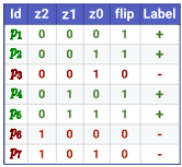
We illustrate PRORP on program Geo0 (Figure 1a) with φ : (z = 0) ∧ (flip = 0), unsigned 3-bit encoding for z, k = 5, and ϵ1 = ϵ2 = 0.2. To generate labeled positive and negative samples, we call FoRT and BaRT with the candidate formula set to False and True respectively, yielding the sample multiset in Figure 1b (every element distinct here), from which we learn a decision tree (Figure 1c). The green (positive) and red (negative) states are compiled into the formula ψ : (z1 ∨ flip) as described in Section 2.3.
The verification-repair loop continues until both checks succeed. In this instance, FoRT produces no counterexamples, while BaRT reports 1100 (denoted by p8) as a Ba-counterexample, raising Error2 from 0.0 to 0.4. TreeRepair considers two repairs of leaf 3: (i) splitting on flip (Figure 1d) or (ii) pruning (Figure 1e), both driving (Error1, Error2) to 0. Assuming the prune mutation is chosen, the resulting tree (Figure 1e) represents flip. Reverification yields a new Ba-counterexample 1101, prompting a refinement (e.g., splitting leaf 2 on z2) that produces the final tree for ψ := (¬z2 ∧ flip). The verification errors now lie within the thresholds (ϵ1, ϵ2) = (0.2, 0.2), and the algorithm terminates.
4.5 Theoretical Guarantee
Theorem 2 (Correctness of PRORP). If PRORP halts, the returned formula ψ represents a (ϵ1, ϵ2, δ)-approximate statistically likely k-step reachable set.
Corollary 1. If PRORP halts and returns the formula ψ, then with probability at least (1 - δ), ϵ1-Clk(φ) ⊆ Rψ.
The formal proof of Theorem 2 is given in the full version [Ray et al., 2026] of this paper.
5 Evaluation
PRORP is implemented in Python using scikit-learn for decision trees, CMSGen [Golia et al., 2021] and Pepin [Soos et al., 2023] for uniform-like CNF/DNF sampling, CadiCaL [Biere et al., 2024] for SAT solving, and Z3 [Moura and Bjørner, 2008] to generate program formula. We evaluate 16 benchmarks from prior work [Bao et al., 2024; Chen et al., 2015; Kaminski and Katoen, 2017] by varying the precondition φ, unroll depth k ∈ {16, 32, 64, 128}, bitwidth (16/32-bit), using ϵ1 = ϵ2 = 0.05, δ = 0.1 and uniform input distribution. We set a timeout of 2 hours. Our experiments address four research questions:
- RQ1: Can PRORP synthesize an (ϵ1, ϵ2, δ)-approximate statistically likely k-step reachable set for a range of programs and preconditions?
- RQ2: Does PRORP scale for many variables and large k?
- RQ3: Do candidate sets synthesized by PRORP correspond to meaningful interpretations?
- RQ4: Is PRORP better than na¨ıve Monte Carlo sampling?
5.1 RQ1: Efficiency of Synthesizing Approximate Statistically Likely k-Step Reachable Set
PRORP successfully produced a candidate formula for the (ϵ1, ϵ2, δ)-approximate k-reachable set on all 218 instances, with runtimes ranging from 6 to 755 seconds for the 16-bit encodings and 6 to 1885 seconds for the 32-bit encodings. We manually verified that, for each problem instance, the candidate set indeed contains the entire ϵ1-Clk(φ) set. Table 2 reports the number of learning phases (#PH), total time (TT) and candidate set obtained for seven illustrative benchmarks with a chosen precondition for 16-bit encoding and unrolling depth k set to 64. The complete and detailed set of experimental results is given in the full version [Ray et al., 2026].
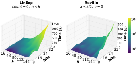
5.2 RQ2: Scalability of PRORP with Respect to k and Bit-Width of Program Variables
To address this question, we selected two representative benchmarks, LinExp and RevBin, each with a single precondition under a uniform input distribution, and measured runtime across varying bit-widths and unrolling depths. Figure 2 reports the resulting performance curves. As expected, runtime increases with both program bit-width and unrolling depth k: larger bit-width blows up the state space exponentially, while higher value of k expands the reachable portion of the state space. From the evaluation results, LinExp incurs the highest runtime cost, exceeding 1000 seconds for large k and bit-width, whereas RevBin exhibits a similar upward trend in runtime but remains under 500 seconds. Overall, these results indicate that PRORP scales predictably across varying bit-widths and unrolling depths for the evaluated programs, within the parameter ranges studied.
| Program | Precondition | k | #PH | TT (secs) | Candidate |
|---|---|---|---|---|---|
| Geo0 | (z14) | 64 | 1 | 6.96 | (z14) |
| LinExp | (count<64) | 64 | 3 | 44.89 | 0≤count<256 |
| Sum0 | (x=64, n< k2 ) | 64 | 4 | 63.80 | 64≤x<512 |
| Fair | (count<64) | 64 | 2 | 21.90 | 0≤count<64 |
| DepRV | (x=0, y=0, n=k) | 64 | 7 | 104.52 | 20≤x<44, y=64-x |
| RevBin | (x= k2 , z<16) | 64 | 4 | 40.58 | 48≤z<80 |
| Mart | (c=0, b=64, r=0) | 64 | 7 | 65.79 | c=64, b=0, 0<r<8 |
5.3 RQ3: Interpretation of the Candidate Sets to Interesting Problems (Case Study)
Let us discuss and interpret the output of PRORP on the program Sum0 [Chen et al., 2015]. The program (Figure 4) has a loop whose number of iterations is fixed by the input variable n. In the i-th iteration the value of x is incremented by (n - i) with probability 12 and not incremented with remaining probability 12 . Here, we consider only preconditions with exactly one satisfying assignment, i.e., (x = x0, n = n0). Note that for Sum0, all terminal states are characterized by n = 0. Let X be the random variable denoting the value of x for terminal states. Thus, E[X] = x0 + n0(n0+1) 4 and X takes values in the interval [x0, x0 + n0(n0+1) 2 ]. That is, if Rφ = {(x0, n0)}, then Clk(φ) := x0 ≤ x ≤ x0 + n0(n0+1) 2 , assuming k ≥ n0. We also note that the random variable X follows a symmetric distribution, with Pr[X = x0 + t] = Pr[X = x0 + n0(n0+1) 2 - t]. In Figure 3 the distribution is plotted for (x0, n0) = (28, 8) which is clearly a bell-shaped curve. Thus, for any ϵ1 ∈ (0, 1], ϵ1-Clk(φ) is of the form (x0 + n0(n0+1) 4 - t ≤ x ≤ x0 + n0(n0+1) 4 + t) which is obtained by chopping off the tails of the distribution.
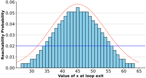
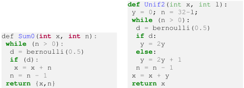
Figure 5: Program Unif2
We observe that the set represented by the output formula is close to ϵ1-Clk(φ). We run PRORP on Sum0 for 4 preconditions with k = 16, each with a single satisfying assignment and parameters ϵ1 = ϵ2 = 0.02 and δ = 0.1. The inputs x and n are 8-bit unsigned integers. The results of our experiment are compiled in Table 3. For each of the 4 preconditions, the right-hand tail of Clk(φ) gets chopped off in Rψ. Also, for two preconditions: {(x = 28, n = 8) and (x = 31, n = 16)}, both the tails of Clk(φ) are trimmed in Rψ and includes the set ϵ1-Clk(φ) fully.
5.4 RQ4: Performance Comparison with Baseline
We evaluate the precision of PRORP against a baseline of na¨ıve Monte Carlo (MC) sampling on a family of 32-bit instances of the benchmark program Unif2 (Figure 5), which returns uniformly distributed values over a configurable interval.
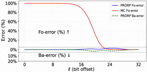
In this family, the reachable set consists of offsets x ∈ [x0, (x0 + 232-ℓ ) mod 232 ) for ℓ = 0, . . . , 32, with precondition φ := (x = x0). We take parameters x0 = 251 and ϵ1 = ϵ2 = 0.05, δ = 0.1, k = 32, and report Fo-error and Ba-error (as percentages) for each ℓ. Figure 6 plots three curves: MC Fo-error, PRORP Fo-error, and PRORP Ba-error (Ba-error is always zero for MC).
In the large-support regime (ℓ ≤ 18), MC yields essentially 100% Fo-error as the sampling budget is overwhelmed by the support size, whereas PRORP attains near-zero Fo and Ba errors. In the transition regime (18 ≤ ℓ ≤ 22), MC Fo-error drops sharply while PRORP incurs minor errors due to tree generalization yet remains substantially more accurate. In the small-support regime (ℓ ≥ 23), both methods achieve negligible error. Overall, PRORP maintains low error across all support sizes, whereas MC becomes competitive only once the reachable support is small enough for exhaustive sampling.
| Rφ | Clk(φ) | ϵ1-Clk(φ) | Rψ |
|---|---|---|---|
| (x = 28, n = 8) | 28 ≤ x ≤ 64 | 36 ≤ x ≤ 56 | 28 ≤ x ≤ 63 |
| (x = 48, n = 16) | 48 ≤ x ≤ 184 | 96 ≤ x ≤ 136 | 48 ≤ x ≤ 175 |
| (x = 31, n = 16) | 31 ≤ x ≤ 167 | 79 ≤ x ≤ 119 | 32 ≤ x ≤ 159 |
| (x = 15, n = 16) | 15 ≤ x ≤ 151 | 63 ≤ x ≤ 103 | 32 ≤ x ≤ 127 |
6 RelatedWork
Probabilistic program analysis is well studied. Exist [Bao et al., 2024], Prinsys [Gretz et al., 2013], Chen et al. [Chen et al., 2015], Feng et al. [Feng et al., 2017], Wang et al. [Wang et al., 2018], MORA [Bartocci et al., 2020], and CegisPro2 [Batz et al., 2023] synthesize quantitative invariants using techniques such as template-based methods, abstract interpretation, and counterexample-guided or data-driven learning. PSI [Gehr et al., 2016] and λPSI [Gehr et al., 2020] compute posterior distributions via computer algebra, while PSE [Geldenhuys et al., 2012] and Plinko [Susag et al., 2022] support symbolic execution of probabilistic programs.
Our work is also related to angelic verification [Das et al., 2015; Das and Lal, 2017; Joshi et al., 2012], which mitigates the pessimism of traditional verification by favoring benign environment behaviors. In contrast, we model the environment probabilistically and learn symbolic summaries of statistically likely reachable states, while guaranteeing that long failure sequences remain improbable.
Methodologically, our approach follows the guess-andcheck paradigm for invariant synthesis. Prior work has used decision trees [Aiken et al., 2016; Ezudheen et al., 2018; Garg et al., 2014; Garg et al., 2016; Riley and Fedyukovich, 2022], PAC learning [Sharma et al., 2013], reinforcement learning [Si et al., 2018; Yu et al., 2023], continuous logic networks [Ryan et al., 2019; Yao et al., 2020], and large language models [Chakraborty et al., 2023; Wu et al., 2024]. Unlike these methods, which synthesize inductive invariants for all reachable states, PRORP learns symbolic summaries of statistically likely reachable states with finite-sample approximation guarantees.
Ethical Statement
This work presents PRORP, a framework for mining statistically likely reachable states in probabilistic programs. The research is purely theoretical and algorithmic in nature, with applications in program verification, AI safety, and bug prioritization. We do not foresee direct negative societal impacts from this work. The benchmarks used in our evaluation are sourced from prior published literature, and no human subjects, private data, or sensitive information were involved in any part of this research.
Acknowledgements
Arijit Ghosh acknowledges partial support from the Science and Engineering Research Board (SERB), Government of India, through the MATRICS grant MTR/2023/001527, and from the Department of Science and Technology (DST), Government of India, through grant TPN-104427. Sourav Chakraborty acknowledges partial support from the TACDCSW/VPP project. This research work was partially supported by Research-I Foundation of IIT Kanpur. Subhajit Roy acknowledges the support of the Jainendra Navlakha (1974) Chair Professorship at IIT Kanpur. Nitesh Trivedi acknowledges the support of FARE Fellowship of IIT Kanpur.
Contribution Statement
Arnab Ray and Nitesh Trivedi contributed equally.
@inproceedings{ijcai2026p712,
  title     = {Mining Statistically Likely k-Reachable States in Probabilistic Programs},
  author    = {Ray, Arnab and Trivedi, Nitesh and Banerjee, Ansuman and Chakraborty, Sourav and Ghosh, Arijit and Roy, Subhajit},
  booktitle = {Proceedings of the Thirty-Fifth International Joint Conference on
               Artificial Intelligence, {IJCAI-26}},
  publisher = {International Joint Conferences on Artificial Intelligence Organization},
  editor    = {Diego Calvanese},
  pages     = {6398--6406},
  year      = {2026},
  month     = {8},
  note      = {Main Track},
  doi       = {10.24963/ijcai.2026/712},
  url       = {https://doi.org/10.24963/ijcai.2026/712},
}
TY - CPAPER TI - Mining Statistically Likely k-Reachable States in Probabilistic Programs AU - Ray, Arnab AU - Trivedi, Nitesh AU - Banerjee, Ansuman AU - Chakraborty, Sourav AU - Ghosh, Arijit AU - Roy, Subhajit T2 - Proceedings of the Thirty-Fifth International Joint Conference on Artificial Intelligence, IJCAI-26 PB - International Joint Conferences on Artificial Intelligence Organization PY - 2026 SP - 6398 EP - 6406 DO - 10.24963/ijcai.2026/712 UR - https://doi.org/10.24963/ijcai.2026/712 ER -Copied
Machine-readable versions of this paper, for tools and AI agents:





