
Extending Weighted Heuristic Search to Bi-Objective Search Problems
Proceedings of the Thirty-Fifth International Joint Conference on Artificial Intelligence. Main Track. Pages 6291-6298.
https://doi.org/10.24963/ijcai.2026/700
Keywords
- Search: Heuristic search
- Search: Combinatorial search and optimisation
Abstract
In heuristic search, a well-known technique to speed up search while providing a suboptimality guarantee is to multiply the heuristic function by a weight w > 1. In this paper, we study the theoretical and practical implications of using such a technique in bi-objective heuristic search, a natural academic exercise that has remained unexplored. We introduce Weighted BOA∗ϵ (WBOA∗
ϵ ), a weighted version of the BOA* algorithm, which uses two real parameters: a weight w for the heuristic and an approximation factor ϵ. Higher values of w and ϵ allow for faster computation of approximate Pareto-optimal solution sets. We prove that WBOA∗ ϵ returns a representative solution set containing (w − 1, ϵ)-approximate solutions. We empirically compare it to A*pex, the state-of-the-art approximate bi-objective search algorithm. We find that WBOA∗ ϵ is competitive with A*pex: when using perfect heuristic functions, in road maps WBOA∗ϵ is faster for higher approximation factors, while in grid maps WBOA∗ϵ dominates A*pex. With imperfect heuristic functions, WBOA∗ϵ performs better than A*pex for lower approximation factors, while the opposite is true for larger approximation factors.
- [Bachmann et al., 2018] Daniel Bachmann, Fritz Bökler, Jakob Kopec, Kira Popp, Björn Schwarze, and Frank We- ichert. Multi-objective optimisation based planning of power-line grid expansions. ISPRS International Journal of Geo-Information, 7(7):258, 2018.
- [Breugem et al., 2017] Thomas Breugem, Twan Dollevoet, and Wilco van den Heuvel. Analysis of fptases for the multi-objective shortest path problem. Computers & Op- erations Research, 78:44-58, 2017.
- [Bronfman et al., 2015] Andrés Bronfman, Vladimir Mari- anov, Germán Paredes-Belmar, and Armin Lüer-Villagra. The maximin hazmat routing problem. European Journal of Operational Research, 241(1):15-27, 2015.
- [Goldin and Salzman, 2021] Boris Goldin and Oren Salz- man. Approximate bi-criteria search by efficient represen- tation of subsets of the pareto-optimal frontier. In Proceed- ings of the 31st International Conference on Automated Planning and Scheduling (ICAPS), pages 149-158, Palo Alto, California, May 2021. AAAI Press.
- [Halle et al., 2025] Yaron Halle, Ariel Felner, Sven Koenig, and Oren Salzman. A preprocessing framework for effi- cient approximate bi-objective shortest-path computation in the presence of correlated objectives. In Proceedings of the 18th International Symposium on Combinatorial Search, pages 65-73, July 2025.
- [Hart et al., 1968] Peter E. Hart, Nils J. Nilsson, and Bertram Raphael. A formal basis for the heuristic determination of minimum cost paths. IEEE Transactions on Systems Science and Cybernetics, 4(2):100-107, July 1968.
- [Hernández et al., 2020] Carlos Hernández, William Yeoh, Jorge A. Baier, Han Zhang, Luis Suazo, and Sven Koenig. A simple and fast bi-objective search algorithm. In Pro- ceedings of the 30th International Conference on Auto- mated Planning and Scheduling (ICAPS), pages 143-151, May 2020.
- [Pohl, 1970] Ira Pohl. Heuristic search viewed as path find- ing in a graph. Artificial Intelligence, 1(3-4):193-204, 1970.
- [Pulido et al., 2015] Francisco-Javier Pulido, Lawrence Mandow, and José-Luis Pérez-de-la-Cruz. Dimension- ality reduction in multiobjective shortest path search. Computers & Operations Research, 64:60-70, 2015.
- [Salzman et al., 2023] Oren Salzman, Ariel Felner, Carlos Hernández, Han Zhang, Shao-Hung Chan, and Sven Koenig. Heuristic-search approaches for the multi- objective shortest-path problem: Progress and research opportunities. In Edith Elkind, editor, Proceedings of the Thirty-Second International Joint Conference on Ar- tificial Intelligence, IJCAI-23, pages 6759-6768. Interna- tional Joint Conferences on Artificial Intelligence Organi- zation, 8 2023. Survey Track.
- [Zhang et al., 2022] Han Zhang, Oren Salzman, T. K. Satish Kumar, Ariel Felner, Carlos Hernández Ulloa, and Sven Koenig. A*pex: Efficient approximate multi-objective search on graphs. In Proceedings of the 32nd Interna- tional Conference on Automated Planning and Scheduling (ICAPS), pages 394-403, Palo Alto, California, June 2022. AAAI Press.
References were extracted automatically from the PDF and may contain errors.
Full text extracted automatically from the PDF; figures, tables and equations may differ. The PDF is the version of record.
1 Introduction
In bi-objective search, we are given a graph G where each edge has an associated pair of costs, an initial state and a goal state. The task is to find a Pareto-optimal solution set, which contains all solution paths (paths that connect the start and goal states) that are not dominated by other solution paths. Bi-objective search is important in AI research. Many realworld decision problems can be represented as an instance of it, such as balancing distance and risk when transporting hazardous materials [Bronfman et al., 2015] or ecological and financial impact when planning power grid expansions [Bachmann et al., 2018].
Finding the Pareto-optimal solution set may be very computationally expensive. Indeed, its size can be exponential in the size of the graph [Breugem et al., 2017]. A key approach to tackle this problem is to compute approximations of the solution set using a relaxed version of dominance called ϵ-dominance [Breugem et al., 2017; Zhang et al., 2022; Goldin and Salzman, 2021; Salzman et al., 2023]. While a path π with cost (c1, c2) weakly dominates path π′ with cost (c′1 , c′2 ) when c1 ≤ c′1 and c2 ≤ c′2 , we say that π ϵdominates path π′ if c1 ≤ (1 + ϵ1)c′1 and c2 ≤ (1 + ϵ2)c′2 , with ϵ = (ϵ1, ϵ2). An intuitive reason why search runs faster with ϵ-dominance is that such a relation allows more pruning than standard dominance.
In this paper, we propose an algorithm to compute approximate Pareto-optimal solution sets drawing inspiration from standard heuristic search. In single-objective search, costs are scalars numbers, and A* [Hart et al., 1968], which uses an Open priority queue with the priority function f(s) = g(s) +h(s), is guaranteed to find optimal solutions when the heuristic function is admissible. In many problems, faster execution times can be obtained when multiplying the heuristic function by a real number w > 1. The resulting algorithm, Weighted A* [Pohl, 1970], can be proven to return solutions whose suboptimality is bounded by w. Despite the practical advantage of weighted heuristics in single-objective search and the fact that algorithms in bi-objective search are based on A*, the theoretical and practical implications of multiplying the heuristic by a positive weight w > 1 in bi-objective search have remained unexplored.
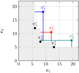
We propose the Weighted Bi-Objective A* (WBOA∗ϵ ) algorithm, which builds on top of the state-of-the-art Bi-Objective A* algorithm [Hern´andez et al., 2020] and its approximate variant BOA∗ϵ [Goldin and Salzman, 2021]. WBOA∗ϵ multiplies the first component of the heuristic by a given scalar parameter w (with w > 1) and can be proven to return a representative approximation of the Pareto-optimal solution set. Specifically, for every optimal path π∗ in the Paretooptimal solution set, there is a solution returned by WBOA∗ϵ that (w-1, ϵ)-dominates π∗ . For an illustration of this property, Figure 1 shows the regions in which WBOA∗ϵ guarantees at least one solution will be found.
We evaluate WBOA∗ϵ on two benchmark domains: DIMACS challenge road maps and Moving AI gridworld maps. For road maps we use perfect heuristic functions computed via Dijkstra's algorithm, while for gridworld maps we evaluate both perfect heuristics and the less informed Octile distance heuristic. WBOA∗ϵ achieves substantial speedups over BOA*; for instance, on the LKS road map with 2,758,119 states, we observe speedups of 96× and 351× when using w = 1.1 and w = 1.2, respectively. In our empirical comparison with A*pex [Zhang et al., 2022], the state-of-theart approximate bi-objective search algorithm, we find that WBOA∗ϵ is competitive across different scenarios. With perfect heuristic functions, WBOA∗ϵ outperforms A*pex on road maps at the highest approximation factors, while on gridworld maps WBOA∗ϵ dominates A*pex across nearly all approximation factors tested. When using the less informed Octile heuristic on gridworld maps, WBOA∗ϵ maintains its advantage at lower approximation factors, though A*pex becomes superior as the approximation factor increases. Additionally, WBOA∗ϵ tends to return fewer solutions than A*pex, which may be preferable in applications where concise solution sets are desired.
2 Notation
Boldface lower case letters are used to represent twocomponent vectors or vectorial functions. For v a vector, v1 and v2 represent the first and second components of v respectively. The addition of two such vectors is defined as v + w = (v1 + w1, v2 + w2). We use v ⪯ w to denote that v weakly dominates w (that is, v1 ≤ w1 and v2 ≤ w2), and v ≺ w to denote that v (strongly) dominates w (that is, v ⪯ w and v1 < w1 or v2 < w2). We also use v ⪯ϵ w if, for a vector of approximation factors ϵ = (ϵ1, ϵ2), v1 ≤ (1 + ϵ1)w1 and v2 ≤ (1 + ϵ2)w2. In this case, we say that v ϵ-dominates w.
A bi-objective search graph is a triple (S,E, c), where S is a set of states, E ⊆ S × S is a set of directed edges and c : E → R+0 × R+0 is a cost function mapping every edge to a pair of non-negative numbers. A path π is a sequence e1, e2, . . . , en of edges in E such that there exists a sequence of states s1, s2, . . . , sn+1 such that ei = (si, si+1), for every i ∈ {1, . . . , n}, which we say starts in s1 and reaches sn+1. We denote the state reached by a non-empty path π by last(π). The symbol λ denotes the empty sequence. The cost of a path π is denoted by c(π) and is defined as the sum of the costs of all edges in π.
A bi-objective search instance is a tuple (S,E, c, sstart, sgoal), where P = (S,E, c) is a bi-objective search graph, and where sstart and sgoal denote, respectively, the start and goal states (in S). A path π is a solution to a problem if its starting state is sstart and its final state is sgoal. A path π is an optimal solution if π is a solution and no other solution π′ is such that π′ ≺ π. The Pareto-optimal solution set for a given instance P contains all optimal solutions to that instance, and is denoted by solsP .
Bi-objective search algorithms utilize heuristic functions, defined as h : S → R≥0×R≥0 . For a state s ∈ S, h(s) serves as an estimate of the minimum cost for each component on all paths from s to sgoal. A heuristic function h is admissible if and only if, for every state s, h(s) ⪯ c(π) for every path π from s to sgoal. A heuristic function h is consistent if and only if h(sgoal) = (0, 0) and h(s) ⪯ c(s, t) + h(t) for all (s, t) ∈ E. Consistency implies admissibility.
3 Background
3.1 Bi-Objective A*
Bi-Objective A* (BOA*) is a state-of-the-art best-first biobjective search algorithm, whose algorithmic design closely resembles A*. BOA* has been shown to have better performance than other bi-objective search algorithms based on A* [Hern´andez et al., 2020].
BOA* uses a priority queue Open, which stores paths in the search graph. 1 Each path π in Open starts in sstart and is associated with an f-value defined as f(π) = c(π) + h(last(π)), where h is a consistent heuristic function.
The execution of BOA* resembles that of A* in that in both a path is extracted from Open (Line 7), the state s reached by such a path is expanded (Line 15), and resulting paths reaching the successors of s are added to Open (Line 20).
Paths in Open are sorted according to their f values in lexicographically ascending order; that is, paths are sorted in ascending order by their first-component cost and, in case of ties, in ascending order by their second-component cost. Together with the fact that h is consistent, such an order guarantees that given any state s in the search graph, paths found by BOA* to s have a non-decreasing c1-value, which in turn allows implementing pruning in constant time by applying dimensionality reduction [Pulido et al., 2015]. Specifically, BOA* keeps, for each state s, a gmin 2 -value that stores the
1 Hern´andez et al. [2020] consider Open as composed by nodes which actually represent paths, albeit efficiently implemented via a state plus a parent pointer. In this paper, we define Open as containing paths rather than nodes, since this allows us to simplify our theoretical analysis. Nevertheless, as we see later, WBOA∗ϵ can be implemented as efficiently as BOA* since it is only different from it in a few lines of code.
Algorithm 1: Bi-Objective A* (BOA*)
Input : A search problem (S,E, c, sstart , sgoal ) and a consistent heuristic function h 1 sols ←Empty list 2 for each s ∈ S do 3 gmin 2 (s) ←∞ 4 f(λ) ←h(sstart ) 5 Initialize Open and insert the empty path λ into it 6 while Open ̸= ∅ do 7 Remove a path π fromOpen with the lexicographically smallest f-value 8 s ← state reached by π or sstart if π is empty 9 if c2(π) ≥ gmin 2 (s) ∨ f2(π) ≥ gmin 2 (sgoal ) then 10 continue 11 gmin 2 (s) ← c2(π) 12 if s = sgoal then 13 Append π to sols 14 continue 15 for each (s, t) ∈ E do 16 π′ ← π, (s, t) 17 f (π′ ) ← c(π′ ) + h(t) 18 if c2(π′ ) ≥ gmin 2 (t) ∨ f2(π′ ) ≥ gmin 2 (sgoal ) then 19 continue 20 Insert π′ to Open 21 return solsc2-value of the last path found that reached s. A path π is pruned either when c2(π) ≥ gmin 2 (last(π)) (local pruning) or when c2(π) ≥ gmin 2 (sgoal ) (global pruning). Hern´andez et al. [2020] show that this form of pruning is sound, which means that a prefix of an optimal solution may be pruned only if another solution of equal cost is returned.
3.2 BOA∗ϵ
Goldin and Salzman [2021] propose a simple modification to BOA* that allows it to compute a subset of the Pareto-optimal solution set. In BOA∗ϵ , the global pruning rule of BOA* is changed to (1 + ϵ)f2(π) ≥ gmin 2 (sgoal ). It can be proven that for any given instance, BOA∗ϵ returns a subset of the solutions returned by BOA* such that no pair of solutions in such a set (0, ϵ)-dominates each other [Goldin and Salzman, 2021].
4 Weighted BOA∗ϵ
Weighted BOA∗ϵ (WBOA∗ϵ ) is obtained by making two simple modifications to BOA∗ϵ . First, it associates the following fvalue to each node in Open.
with w > 1. Second, we replace Line 13 in Algorithm 1 with Algorithm 2. WBOA∗ϵ is conceptually simple because it requires almost no additional modification with respect to BOA*. In contrast, A*pex [Zhang et al., 2022], the stateof-the-art approximate search algorithm for bi-objective (and multi-objective) search problems, has to check if it can merge two paths at each step. This checking technique provides a performance advantage to A*pex when there are many similarities between paths [Zhang et al., 2022], but it comes with computational overhead.
Algorithm 2: Handling new solutions in WBOA∗ϵ
1 while |sols| > 0 and c1(last(sols)) ≥ c1(π) do 2 Remove the last element from sols- 3 Append π to sols
Before we continue with the theoretical analysis, we make two important observations. Firstly, in the definition of f w , the second component is not affected by w. There are two reasons for this. First, BOA∗ϵ already has an approximation factor associated with the second component and thus by not changing f's second component we allow the theoretical properties of BOA∗ϵ to be leveraged by WBOA∗ϵ (see Theorem 1). Second, from a practical perspective, inWBOA∗ϵ , like BOA*, Open is sorted lexicographically and thus the weight w affects search mainly in the first component, since the second component of f w is only used as a tiebreaker.
The second observation is that WBOA∗ϵ , in practice, does not use a consistent heuristic even if its input heuristic h is consistent, since multiplying the first component of h by w can make its first component inconsistent. This implies that an important property of BOA∗ϵ is broken: paths to a given state s are not guaranteed to be found in monotonically nondecreasing c1 order.
One implication of using a non-monotonic f function is that BOA∗ϵ 's technique of using gmin 2 value of s to prune in constant time does not allow pruning all dominated paths to s. This means that while a path π may be initially found to a certain state, subsequently another path π′ may be found to the same state such that c1(π′ ) < c1(π) while at the same time c2(π′ ) < c2(π). Even though this means that π′ dominates π, WBOA∗ϵ does not prune π from Open. This is why WBOA∗ϵ uses Algorithm 2 to filter out dominated paths from the returned solution set. Observe that after running Algorithm 2, the paths in sols remain sorted by ascending c1-value. This, together with the local pruning rule, which still guarantees that solutions found have a decreasing c2 cost, ensures that sols contains a set of non-dominated paths.
While BOA* never prunes a prefix of an optimal path from Open, WBOA∗ϵ can do so, which is important to note since it influences our theoretical analysis. Indeed, consider that π is a path that passes through state u; for simplicity, let us represent π as the concatenation of two paths π1π2 where π1 is the sequence that reaches state u. Since f w is non-monotonic, during the execution of WBOA∗ϵ it may be possible to extract a path ρ to u, before extracting π1, even if c1(ρ) > c1(π1). After finding ρ, gmin 2 (u) is set to c2(ρ). If it is also the case that c2(ρ) < c2(π1) then, due to the local pruning rule, π will be pruned if it is ever extracted fromOpen, meaning the optimal solution π will not be found.
4.1 An Example Execution
Figure 2 and Table 1 show an example of an execution of WBOA∗ϵ over a search graph, using the parameters w = 2 and ϵ = 1. For the execution, we consider a perfect heuristic distance, which can be computed using Dijkstra's algorithm. For ease of understanding, in this section we represent a path (s1, s2) . . . (sn-1, sn) by its sequence of states in the form of s1→s2 → . . .→sn-1→sn. Although the Pareto-optimal paths of the search instance are sstart→s1→s4→sgoal (with a cost of (8, 10)) and sstart→s3→sgoal (with a cost of (11, 6)), neither of these is returned by the algorithm as their prefixes end up being pruned. The events in each iteration of the algorithm are as follows:
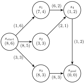
- The initial empty path λ at sstart is expanded, adding to the Open list the paths sstart→s1, sstart→s2, and sstart→s3.
- sstart→s2 is expanded. gmin 2 (s2) is set to 5 and sstart→s2→s4 is added to Open.
- sstart→s2→s4 is expanded. gmin 2 (s4) is set to 6, which means that the path sstart→s1, if expanded, will have its only successor be locally pruned. sstart→s2→s4→sgoal is added to Open.
- sstart→s2→s4→sgoal is expanded and found as a solution with a cost of (11, 8). gmin 2 (sgoal ) is set to 8.
- sstart→s1 is extracted from open. As it has a f w 2 value of 10 and gmin 2 (sgoal ) = 8, it is pruned according to the global prune no matter the value of ϵ.
- sstart→s3 is extracted from open. As it has a f w 2 value of 6, gmin 2 (sgoal ) = 8, and ϵ = 1, it is pruned according to the global prune because (1 + 1) · 6 ≥ 8.
- Finally, as Open is empty, the execution of WBOA∗ϵ finishes. The approximate Pareto-optimal solution set returned is the single solution path sstart→s2→s4→sgoal .
5 Theoretical Results
In this section we prove our main theoretical result. Based on the previous discussion, in which we saw that optimal paths may be pruned by a run of WBOA∗ϵ , we formally define when a solution path locally prunes another solution path, a notion that is useful later for our proof.
Definition 1. Given an execution of WBOA∗ϵ over a biobjective search instance P we say that path π is locally pruned by path ρ if and only if:
- both π and ρ reach a common intermediate state u, from where they continue with the same path. Formally, π =
- π′σ and ρ = ρ′σ, such that both π′ and ρ′ reach the same state u;
- during execution, path ρ′ is extracted fromOpen before π′ and not pruned, while a (not necessarily proper) prefix of π′ is in Open; finally,
| w = 2, ϵ = 1 | ||
|---|---|---|
| Iteration | Open list (last(π), g(π), f w (π)) | Update of gmin 2 (s(π)) |
| 1 | (sstart , (0, 0), (16, 6)) ← | gmin 2 (sstart ) = 0 |
| 2 | (s1, (1, 6), (15, 10)) (s2, (8, 5), (14, 8)) ← (s3, (3, 3), (19, 6)) | gmin 2 (s2) = 5 |
| 3 | (s1, (1, 6), (15, 10)) (s3, (3, 3), (19, 6)) (s4, (10, 6), (12, 8)) ← | gmin 2 (s4) = 6 |
| 4 | (s1, (1, 6), (15, 10)) (s3, (3, 3), (19, 6)) (sgoal , (11, 8), (11, 8)) ← | gmin 2 (sgoal ) = 8 |
| 5 | (s1, (1, 6), (15, 10)) ← (s3, (3, 3), (19, 6)) | |
| 6 | (s3, (3, 3), (19, 6)) ← | |
| 7 | empty | |
Additional notation To simplify presentation, in the remainder of the proof we assume that if π is a path and h is a heuristic function, then h(π) abbreviates the notation h(sπ), where sπ is the state reached by π. Furthermore, if a path π is the concatenation of ρ and σ, then the notation π-σ corresponds to removing the suffix σ from π; therefore π -σ = ρ.
We start off our theoretical analysis with Lemma 1, which is a standard result of consistent heuristics.
Lemma 1. Let π1 and π2 be paths such that π1π2 is also a path. Then h(π1) ≤ c(π2) + h(π1π2).
Our first original theoretical result below shows that whenever a path is locally pruned by another path, then the pruner path's cost (w - 1, 0)-dominates the pruned path's cost. This holds, in particular, when the pruned path is an optimal path.
Lemma 2. In an execution of WBOA∗ϵ , if π1, π2, . . . , πn is a sequence of paths such that πi+1 locally prunes πi, for every i ∈ {1, . . . , n - 1}, then c(πn) ⪯(w-1,0) c(π1).
Proof. The proof is by induction on n. For the base case, n = 1, we have trivially c(π1) ⪯(w-1,0) c(π1).
For the induction, we assume the property holds for n = k, and we prove for n = k + 1. Since c(πk) ⪯(w-1,0) c(π1), we have:
To prove c(πk+1) ⪯(w-1,0) c(π1) we need to prove the two inequalities:
We start by proving (4). Observe that, by Definition 1, since πk+1 locally prunes πk, c2(πk+1) ≤ c2(πk), which, together with (2), implies (4).
We continue with the proof for (3). From Definition 1, we know that πk+1 and πk share a common suffix; therefore πk = ρkσ and πk+1 = ρk+1σ, where both ρk and ρk+1 reach the same state uk. Because ρk+1 locally prunes ρk at state uk, we observe that a (not necessarily proper) prefix of ρk, say ρ′k , is in Open at the time ρk+1 is extracted; that is ρk = ρ′k ρ′′ k . At that point in execution f w 1 (ρk+1) ≤ f w 1 (ρ′k ), thus:
Observe that the sequence of k paths given by:
where τi = πi - ρ′′ k σ is also such that τi+1 locally prunes τi, for every i ∈ {1, . . . , k - 1}. 2 Therefore, we apply the inductive hypothesis over the sequence in (6) and obtain:
Now we instantiate Lemma 1 as follows:
By adding (5), (7) and the multiplication of (8) by w, and by using the fact that h1(ρk+1) = h1(ρ′′ k ), since both ρk+1 and ρ′′ k reach the same state, we obtain:
Now we add c1(σ) to the left-hand side of (9) and wc1(σ) to the right-hand side of (9) and obtain the desired result.
Theorem 1. Let π∗ be an optimal solution to a bi-objective search instance P . Then the solution set returned by WBOA∗ϵ over P contains a path that (w - 1, ϵ)-dominates π∗ .
Proof. An execution of WBOA∗ϵ defines a sequence of paths ρ1, ρ2, . . . , ρn (n ≥ 1) such that ρ1 = π∗ and ρi+1 locally prunes ρi, for every i ∈ {1, . . . , n - 1}, and such that ρn is not locally pruned by any other path. From Lemma 2,
If ρn is in the solution set returned by WBOA∗ϵ , then the result is straightforward since Inequality (10) implies c(ρn) ⪯(w-1,ϵ) c(π∗ ).
If ρn is not in the solution set returned by WBOA∗ϵ , then a prefix ρ′n of ρn is pruned by the global pruning rule. Therefore, when ρ′n is extracted, there is a solution π in sols, such that:
2 Note that all paths π1, . . . , πk share a common suffix representing the path from the state uk-1 (where πk-1 was locally pruned) to last(π1). As the local pruning of πk occurs after that of πk-1, the state uk-1 is traversed in ρ′k and ρ′′ kσ is a suffix of all paths π1, . . . , πk.
Because h is admissible, Inequality (11) implies:
In addition, when WBOA∗ϵ extracts π from Open there is a prefix of ρn, ρ′′n in Open such that f w 1 (π) ≤ f w 1 (ρ′′n ). This implies that c1(π) ≤ c1(ρ′′n ) +wh1(ρ′′n ). By admissibility of h:
Inequalities (12) and (13) imply:
In turn, (10) and (14) imply:
Finally, after ρn is globally pruned by π in sols, it could be the case that π is removed from sols by another solution π2, and later on π2 removed by π3, and so on and so forth. More formally π1, . . . , πm can be a sequence of solutions such that π1 = π, and πi+1 removes πi from sols via Algorithm 2, and πm is not removed by any solution and therefore πm ∈ sols when sols is returned. But Algorithm 2 guarantees that c(πi+1) ≺ c(πi). Thus, c(πm) ⪯ c(π) , which together with (15) yields c(πm) ⪯(w-1,ϵ) c(π∗ ), which is what we wanted to prove.
6 Experimental Results
We compared WBOA∗ϵ to the approximate multi-objective search algorithm A*pex, 3 as it has recently been shown to be the most efficient algorithm of the state of the art and surpasses even dedicated bi-objective algorithms like PP-A* [Goldin and Salzman, 2021]. A*pex uses two approximation factors (ϵ1, ϵ2) as its parameters for bi-objective search, each corresponding to their respective objective.
We ran all tests on a Linux machine with a 4.4GHz Intel ® Core™ i5-12400 CPU and 32GB RAM. WBOA∗ϵ was implemented in C++ 4 and we used the C++ implementation of A*pex provided by the authors. To compare the algorithms, we used the standard road maps benchmarks obtained from the 9th DIMACS Implementation Challenge - Shortest Paths 5 , with the cost components representing travel distance (c1) and time (c2). We compare the algorithms in two large maps of the dataset. We used 76 search instances of LKS road map and 50 instances of CAL road map, which represent the available queries that ran to completion for every approximation value with both algorithms. Additionally, we used 8-neighbor grid maps from the Moving AI Lab repository, 6 with c1 representing travel distance and c2 being a random number between 1 and 6. We compare the algorithms in two maps of size 1024×1024 (Expedition and Paris-1) and in two maps of size 512×512 (Random-512-20-0 and Maze-512-160). We used 50 random search instances for each map.
3 There exist three main implementations of A*pex which vary in merge strategy. We use the Greedy variant as described by Zhang et al. [2022], as this one tends to be superior in their evaluation.
4 https://github.com/hansjkl/WBOAE
5 https://www.diag.uniroma1.it/challenge9/download.shtml
6 https://movingai.com/benchmarks/grids.html
(e) Expedition map, Octile
(f) Random map, Octile
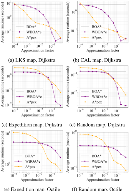
Figure 3: Average runtimes of WBOA∗ϵ and A*pex across all instances for a given map and heuristic plotted against ϵ′ .
The heuristic h used corresponds to the exact minimum travel distances and minimum travel times to sgoal , computed using Dijkstra's algorithm. In grid maps, we also run experiments with the Octile distance. For h1 we used the standard Octile distance and for h2 we use a cost equal to one for both orthogonal and diagonal moves. The computation time of h is omitted from the reported runtime of each test, as both algorithms compute it in the same manner. To provide equivalent theoretical guarantees from both algorithms, we use a single approximation factor ϵ′ > 0 so that WBOA∗ϵ uses parameters (w = 1 + ϵ′ , ϵ = ϵ′ ) and A*pex uses ϵ = (ϵ′ , ϵ′ ). We evaluated 11 ϵ′ values: 0.0001, 0.0005, 0.001, 0.002, 0.005, 0.01, 0.02, 0.05, 0.1, 0.2, and 0.5.
6.1 Runtime
Figure 3 shows the average runtime of both algorithms on all search instances for each map and each approximation value tested. For the grid maps, we have chosen Expedition and Random as representatives, because the results from Paris and Maze512 are similar. We observed that when the algorithms used a Dijkstra (i.e., perfect) heuristic function on road maps A*pex outperform WBOA∗ϵ in most of the ϵ values evaluated (7 of 11 values), and on grid maps the opposite occurs: WBOA∗ϵ outperforms A*pex on 10 out of the 11 ϵ values evaluated. When the algorithms were run with the Octile heuristic function on the grid maps, we observed that WBOA∗ϵ outperforms A*pex for the 6 smaller ϵ values evaluated, and A*pex outperforms WBOA∗ϵ for the remaining values.
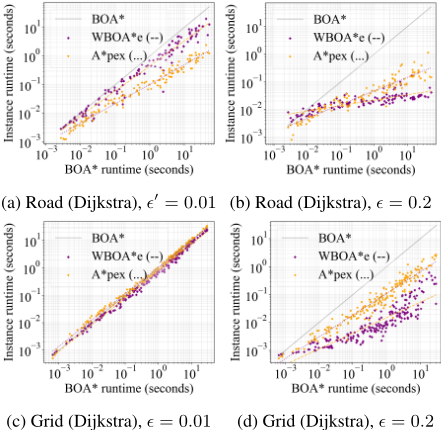
Figure 4 shows the runtimes of each instance using a Dijkstra heuristic for values of ϵ′ ∈ {0.01, 0.2}, sorted along the x-axis in ascending order according to the runtime of BOA* for each. We observed that on road maps with ϵ′ equal to 0.01, A*pex is faster thanWBOA∗ϵ in most of the instances, and on grid maps the opposite happens. On the other hand, with ϵ′ equal to 0.2, WBOA∗ϵ is faster than A*pex in road and grid maps in almost all instances. Figure 4b also shows us that for some approximation values, such as 0.2, WBOA∗ϵ scales better than A*pex as the runtime of BOA* increases.
These differences in performance by map type and heuristic arise from the different pruning mechanisms of each algorithm. A*pex acts on a local level by merging paths which share a last state, which means that graphs where each state has a higher degree (such as grid maps, where states usually have degree 7 or 8) lead to paths in Open less often sharing a final state during the execution of the algorithm, allowing for fewer path mergers. Meanwhile, maps with lower state degrees (such as road maps, with degrees around 2 or 3) allow for more mergers and better time optimization. Similarly, as A*pex relies on the merger of paths in Open, the exact path extraction order as determined by the used heuristic is less likely to stop pruning. Furthermore, the cost components in DIMACS road maps have been shown to have a strong positive correlation [Halle et al., 2025], which allows A*pex to more easily merge paths even while using lower approximation factors. WBOA∗ϵ , meanwhile, executes its local prunes according to a locally determined gmin 2 value, which means high-quality paths being extracted early are vital for efficient pruning. The algorithm also allows for paths to be explored in depth according to the given weight to allow solutions to be found earlier, which means the global pruning can act earlier
- (c) Expedition map, Dijkstra (d) Randommap, Dijkstra
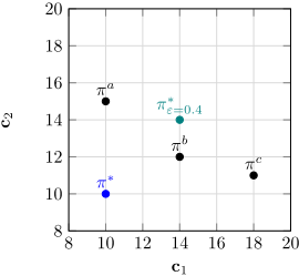
Figure 6: An optimal solution π∗ and an example approximate Pareto-optimal solution set {πa , πb , πc }. The point π∗ ε=0.4 shows the costs of the optimal solution multiplied by 1.4. Such a point is dominated by πb , so we know that πb (0.4, 0.4)-dominates π∗ .
in a map with higher degree states when compared to A*pex.
6.2 Number and quality of solutions
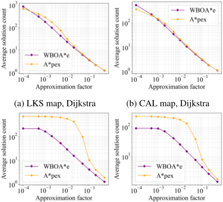
Figure 5 shows the average solution quantity found by both algorithms for each map and approximation factor. We observe that WBOA∗ϵ tends to return fewer solutions than A*pex, for each search instance, with the difference being more pronounced for grid maps.
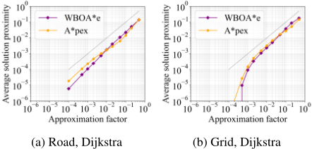
We evaluate the quality of a returned solution set using socalled proximity values. Formally, the proximity value of an optimal solution path π∗ with respect to a solution set S is the smallest real number ε such that there exists one path π in S such that c(π) ⪯(ε,ε) c(π∗ ). To illustrate this concept, Figure 6 shows an optimal solution π∗ and a set of found solutions, with the smallest possible value for ε being 0.4.
To evaluate the quality of an approximate solution set S, we average the proximity value of every solution path π in a Pareto-optimal solution set with respect to S. Figure 7 shows the average proximity value of all found solution sets for each algorithm and approximation factor in both types of map. We generally see WBOA∗ϵ finding more representative solutions for lower approximation factors, while A*pex gains an advantage at higher values such as 0.05, 0.1, 0.2 and 0.5.
7 Summary and Conclusions
We introduced Weighted BOA∗ϵ (WBOA∗ϵ ), a novel approximate bi-objective search algorithm that extends the weighted heuristic technique from single-objective search to the biobjective setting. Our approach builds on the state-of-theart BOA* algorithm and its approximate variant BOA∗ϵ by multiplying the first component of the heuristic function by a weight w > 1. This simple modification, combined with an approximation factor ϵ, enables faster computation of approximate Pareto-optimal solution sets while providing theoretical guarantees on solution quality. We prove WBOA∗ϵ returns a (w - 1, ϵ)-representative solution set. This result establishes a relationship between the weight parameter and the approximation quality, filling a gap in the literature where weighted heuristics had not been studied in bi-objective search.
Our experimental evaluation compared WBOA∗ϵ against A*pex, the current state-of-the-art approximate bi-objective search algorithm, across two benchmark domains: DIMACS road maps and Moving AI gridworld maps. The results show that WBOA∗ϵ is competitive with A*pex, with performance depending on map characteristics, heuristic quality, and approximation factors. The performance differences can be attributed to the distinct mechanisms of the two algorithms. A*pex operates through local path merging, which benefits from lower state degrees and correlated cost components, while WBOA∗ϵ relies on global pruning with gmin 2 values, which excels when high-quality paths are explored early and when state degrees are higher.
Our proximity analysis to measure quality of the solution set showed that WBOA∗ϵ finds better-quality solution sets at lower approximation factors, while A*pex can be closer to the Pareto-optimal solution set at higher factors. Additionally, WBOA∗ϵ generally returns fewer solutions than A*pex, which may be advantageous in scenarios where concise solution sets are preferred.
Acknowledgements
Jorge A. Baier and Carlos Hern´andez are grateful to the National Center for Artificial Intelligence CENIA FB210017, Basal ANID. The research at the University of California, Irvine and the University of Southern California was supported by the National Science Foundation (NSF) under grant numbers 2544613, 2434916, and 2321786, as well as gifts from the Donald Bren Foundation. This research was supported by the United States-Israel Binational Science Foundation (BSF) grants no. 2021643. The work of Ariel Felner was supported by the Israel Science Foundation (ISF) grant #909/23.
@inproceedings{ijcai2026p700,
  title     = {Extending Weighted Heuristic Search to Bi-Objective Search Problems},
  author    = {Kühn Leiva, Hans and Baier, Jorge A. and Hernandez Ulloa, Carlos and Salzman, Oren and Felner, Ariel and Koenig, Sven},
  booktitle = {Proceedings of the Thirty-Fifth International Joint Conference on
               Artificial Intelligence, {IJCAI-26}},
  publisher = {International Joint Conferences on Artificial Intelligence Organization},
  editor    = {Diego Calvanese},
  pages     = {6291--6298},
  year      = {2026},
  month     = {8},
  note      = {Main Track},
  doi       = {10.24963/ijcai.2026/700},
  url       = {https://doi.org/10.24963/ijcai.2026/700},
}
TY - CPAPER TI - Extending Weighted Heuristic Search to Bi-Objective Search Problems AU - Kühn Leiva, Hans AU - Baier, Jorge A. AU - Hernandez Ulloa, Carlos AU - Salzman, Oren AU - Felner, Ariel AU - Koenig, Sven T2 - Proceedings of the Thirty-Fifth International Joint Conference on Artificial Intelligence, IJCAI-26 PB - International Joint Conferences on Artificial Intelligence Organization PY - 2026 SP - 6291 EP - 6298 DO - 10.24963/ijcai.2026/700 UR - https://doi.org/10.24963/ijcai.2026/700 ER -Copied
Machine-readable versions of this paper, for tools and AI agents:





