
A Foundation Model for Zero-Shot Logical Rule Induction
Proceedings of the Thirty-Fifth International Joint Conference on Artificial Intelligence. Main Track. Pages 3999-4007.
https://doi.org/10.24963/ijcai.2026/445
Keywords
- Machine Learning: Foundation models
- Machine Learning: Neuro-symbolic methods/Abductive Learning
- Knowledge Representation and Reasoning: Learning and reasoning
- Knowledge Representation and Reasoning: Logic programming
Abstract
Inductive Logic Programming (ILP) learns interpretable logical rules from data. Existing methods are transductive: their learned parameters are bound to specific predicates and require retraining for each new task. We introduce Neural Rule Inducer (NRI), a pretrained model for zero-shot rule induction. Rather than encoding literal identities, NRI represents literals using domain-agnostic statistical properties such as class-conditional rates, entropy, and co-occurrence, which generalize across variable identities and counts without retraining. The model consists of a statistical encoder and a parallel slot-based decoder. Parallel decoding preserves the permutation invariance of logical disjunction; an autoregressive decoder would instead impose an arbitrary clause order. Product T-norm relaxation makes rule execution differentiable, allowing end-to-end training on prediction accuracy alone. We evaluate NRI on rule recovery, robustness to label noise and spurious correlations, and zero-shot transfer to real-world benchmarks, and we believe this work opens up the possibility of foundation models for symbolic reasoning. Code and the reference checkpoint are available at https://github.com/phuayj/neural-rule-inducer. An extended version with full appendices is available at https://arxiv.org/abs/2605.04916.
- [Asuncion et al., 2007] Arthur Asuncion, David Newman, et al. Uci machine learning repository, 2007.
- [Bommasani, 2021] Rishi Bommasani. On the opportu- nities and risks of foundation models. arXiv preprint arXiv:2108.07258, 2021.
- [Cortes and Vapnik, 1995] Corinna Cortes and Vladimir Vapnik. Support-vector networks. Machine learning, 20(3):273-297, 1995.
- [Cropper and Morel, 2021] Andrew Cropper and Rolf Morel. Learning programs by learning from failures. Machine Learning, 110(4):801-856, 2021.
- [Evans and Grefenstette, 2018] Richard Evans and Edward Grefenstette. Learning explanatory rules from noisy data. Journal of Artificial Intelligence Research, 61:1-64, 2018.
- [Fedus et al., 2022] William Fedus, Barret Zoph, and Noam Shazeer. Switch transformers: Scaling to trillion param- eter models with simple and efficient sparsity. Journal of Machine Learning Research, 23(120):1-39, 2022.
- [Gao et al., 2024] Kun Gao, Katsumi Inoue, Yongzhi Cao, and Hanpin Wang. A differentiable first-order rule learner for inductive logic programming. Artificial Intelligence, 331:104108, 2024.
- [Hollmann et al., 2023] Noah Hollmann, Samuel Müller, Katharina Eggensperger, and Frank Hutter. Tabpfn: A transformer that solves small tabular classification prob- lems in a second. In International Conference on Learning Representations 2023, 2023.
- [Inoue et al., 2014] Katsumi Inoue, Tony Ribeiro, and Chi- aki Sakama. Learning from interpretation transition. Ma- chine Learning, 94(1):51-79, 2014.
- [Johnson et al., 2025] Blair Johnson, Clayton Kerce, and Faramarz Fekri. Glidr: Graph-like inductive logic pro- gramming with differentiable reasoning. arXiv preprint arXiv:2508.06716, 2025.
- [Klement et al., 2013] Erich Peter Klement, Radko Mesiar, and Endre Pap. Triangular norms, volume 8. Springer Science & Business Media, 2013.
- [Manhaeve et al., 2018] Robin Manhaeve, Sebastijan Du- mancic, Angelika Kimmig, Thomas Demeester, and Luc De Raedt. Deepproblog: Neural probabilistic logic pro- gramming. Advances in Neural Information Processing Systems, 31, 2018.
- [Muggleton and De Raedt, 1994] Stephen Muggleton and Luc De Raedt. Inductive logic programming: Theory and methods. The Journal of Logic Programming, 19:629- 679, 1994.
- [Muggleton, 1995] Stephen Muggleton. Inverse entailment and progol. New generation computing, 13(3):245-286, 1995.
- [Olausson et al., 2023] Theo Olausson, Alex Gu, Ben Lip- kin, Cedegao Zhang, Armando Solar-Lezama, Joshua Tenenbaum, and Roger Levy. Linc: A neurosymbolic ap- proach for logical reasoning by combining language mod- els with first-order logic provers. In Proceedings of the 2023 Conference on Empirical Methods in Natural Lan- guage Processing, pages 5153-5176, 2023.
- [Peng et al., 2025] Yifei Peng, Yaoli Liu, Enbo Xia, Yu Jin, Wang-Zhou Dai, Zhong Ren, Yao-Xiang Ding, and Kun Zhou. Abductive logical rule induction by bridging in- ductive logic programming and multimodal large language models. arXiv preprint arXiv:2509.21874, 2025.
- [Perez et al., 2018] Ethan Perez, Florian Strub, Harm de Vries, Vincent Dumoulin, and Aaron Courville. Film: Visual reasoning with a general conditioning layer. In AAAI Conference on Artificial Intelligence, pages 3942- 3951, 2018.
- [Phua and Inoue, 2024] Yin Jun Phua and Katsumi Inoue. Variable assignment invariant neural networks for learning logic programs. In International Conference on Neural- Symbolic Learning and Reasoning (NeSy). Springer, 2024.
- [Quinlan, 1990] J. Ross Quinlan. Learning logical defini- tions from relations. volume 5, pages 239-266. Springer, 1990.
- [Ren et al., 2025] ZZ Ren, Zhihong Shao, Junxiao Song, Huajian Xin, Haocheng Wang, Wanjia Zhao, Liyue Zhang, Zhe Fu, Qihao Zhu, Dejian Yang, et al. Deepseek-prover- v2: Advancing formal mathematical reasoning via re- inforcement learning for subgoal decomposition. arXiv preprint arXiv:2504.21801, 2025.
- [Rocktäschel and Riedel, 2017] Tim Rocktäschel and Sebas- tian Riedel. End-to-end differentiable proving. volume 30, 2017.
- [Sadeghian et al., 2019] Ali Sadeghian, Mohammadreza Ar- mandpour, Patrick Ding, and Daisy Zhe Wang. Drum: End-to-end differentiable rule mining on knowledge graphs. Advances in neural information processing sys- tems, 32, 2019.
- [Serafini and Garcez, 2016] Luciano Serafini and Ar- tur d'Avila Garcez. Logic tensor networks: Deep learning and logical reasoning from data and knowledge. 2016.
- [Srinivasan, 2001] Ashwin Srinivasan. The aleph manual. 2001.
- [Vaswani et al., 2017] Ashish Vaswani, Noam Shazeer, Niki Parmar, Jakob Uszkoreit, Llion Jones, Aidan N Gomez, Łukasz Kaiser, and Illia Polosukhin. Attention is all you need. volume 30, 2017.
- [Wang and Gupta, 2022] Huaduo Wang and Gopal Gupta. FOLD-R++: A scalable toolset for automated inductive learning of default theories from mixed data. In Functional and Logic Programming -16th International Symposium, FLOPS 2022, Kyoto, Japan, May 10-12, 2022, Proceed- ings, Lecture Notes in Computer Science, pages 224-242.
- [Yang et al., 2017] Fan Yang, Zhilin Yang, and William W Cohen. Differentiable learning of logical rules for knowl- edge base reasoning. Advances in neural information pro- cessing systems, 30, 2017.
- [Yang et al., 2020] Zhun Yang, Adam Ishay, and Joohyung Lee. Neurasp: Embracing neural networks into answer set programming. In 29th International Joint Conference on Artificial Intelligence (IJCAI 2020), 2020. IJCAI
References were extracted automatically from the PDF and may contain errors.
Full text extracted automatically from the PDF; figures, tables and equations may differ. The PDF is the version of record.
1 Introduction
Inductive Logic Programming (ILP) systems learn interpretable logical rules purely from examples. For example, an ILP system analyzing patient records with symptoms and diagnoses might induce a rule: "(fever ∧ cough) ∨ (chills ∧ body aches) → flu." In high-stakes domains like healthcare and finance, black-box predictions are unacceptable. Transparent logical rules like this give us insights that we can actually trust and use.
Traditional symbolic ILP methods like [Muggleton and De Raedt, 1994; Quinlan, 1990; Srinivasan, 2001; Inoue et al., 2014; Muggleton, 1995; Cropper and Morel, 2021] are sensitive to noise and often have to compromise between precision and coverage. Recently, differentiable approaches such as [Evans and Grefenstette, 2018; Gao et al., 2024; Johnson et al., 2025] have been proposed. These methods have proven to be more robust to noise but they are still transductive, where learned weights are tied to specific predicates. A model trained on family relationships (Parent, Grandparent) cannot be transferred to biology (Protein, Enzyme). This means that for every new dataset, we need to retrain the models from scratch.
So how do we determine which variable (boolean attributes like fever, cough) is predictive of a label (targets like flu)? We select variables by their statistical signatures rather than by name. Because these signatures are invariant to renaming and reordering and each literal is represented by a fixed-dimensional vector independent of N, they offer a plausible route to zero-shot transfer. A high class-conditional rate indicates a variable belongs in a rule, regardless of what it represents. In this paper we test this hypothesis by pretraining on synthetic DNFs and evaluating on held-out real-world tabular tasks without retraining.
This approach requires addressing three challenges. First, variable-sized problems: generalization from fixed-size training data to problems with fewer or more variables. Second, inter-variable dependencies: individual statistics miss redundancy and complementarity (e.g., XOR patterns). Third, synthetic-to-real transfer: learning the abstract procedure of induction rather than overfitting to synthetic data.
We present Neural Rule Inducer (NRI), a foundation model [Bommasani, 2021] that consists of the following:
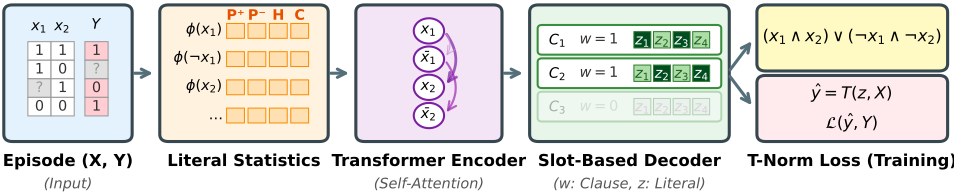
- Literal Statistics Encoder encodes literals by statistical properties such as how often the literal is true and cooccurrences with other literals.
- Parallel Slot-Based Decoder. This module synthesizes multiple clauses in parallel using learned slot queries. Compared to autoregressive models, this module preserves the permutation invariance of logical disjunction.
- T-Norm Training. We use product t-norm relaxation to execute rules differentiably. This allows end-to-end training without explicit clause supervision.
- Synthetic Data Training. We train entirely on randomly generated boolean formulas. This trains the model to recognize the induction procedure itself rather
than domain-specific patterns, and removes the limitation on training data size.
We show that a model trained entirely on synthetic boolean formulas can perform zero-shot rule induction on diverse real-world benchmarks. Figure 1 illustrates the overall architecture of NRI. While in this work, we focus on boolean variables, the statistical encoding framework can be extended to multi-valued and continuous domains via discretization or fuzzy predicates.
2 RelatedWorks
Differentiable ILP. [Evans and Grefenstette, 2018] proposed learning rules via gradient descent, but their method requires specifying rule templates and a fixed set of background predicates. NeuralLP [Yang et al., 2017] and DRUM [Sadeghian et al., 2019] extended this to knowledge base reasoning using TensorLog. Neural Theorem Provers [Rockt¨aschel and Riedel, 2017] introduced differentiable unification for end-to-end theorem proving. Logic Tensor Networks [Serafini and Garcez, 2016] use fuzzy semantics to integrate logical constraints into neural learning. DeepProbLog [Manhaeve et al., 2018] extends probabilistic logic programming with neural predicates, enabling endto-end learning of both neural and symbolic components. NeurASP [Yang et al., 2020] integrates neural networks with answer set programming, allowing neural network outputs to serve as probabilistic inputs to logic programs. GLIDR [Johnson et al., 2025] generalized this to graph-like topologies, utilizing differentiable message passing to learn recursive and cyclic dependencies.
Most differentiable ILP systems instantiate parameters against a fixed predicate or schema inventory, so transferring to a new dataset typically requires retraining. Classical symbolic systems such as FOLD-R++ [Wang and Gupta, 2022], which learns answer-set rules frommixed numerical and categorical data by top-down heuristic search, are similarly taskspecific and are re-run from scratch on each new task.
Phua and Inoue [Phua and Inoue, 2024] proposed a model allowing zero-shot transfer learning. They addressed scaling issues by exploiting variable permutation symmetries. Our proposed method differs in mechanism where instead of utilizing the raw examples, we utilize statistical properties to handle missing and noisy data.
GenerativeNeuro-SymbolicAI. LLM-basedmethods like ILP-CoT [Peng et al., 2025] and DeepSeek-Prover-V2 [Ren et al., 2025] generate hypotheses by relying on knowledge encoded in language and human concepts. LINC [Olausson et al., 2023] combines language models with first-order logic provers, using LLMs to translate natural language into formal logic for external verification. However, LLMs are not grounded in reality, they may use abstract symbols or notions that might not correspond to any measurable quantity in the real world. In contrast, our approach generates hypotheses directly from observed data and does not assume an explicit semantic model. TabPFN [Hollmann et al., 2023] demonstrated that transformers trained on synthetic tabular data can perform in-context learning for classification. While TabPFN
produces black-box predictions, our approach outputs interpretable logical rules.
3 Background
We want to learn a function f : (X, Y) → R that takes input examples X (boolean variables) and labels Y and outputs a logical hypothesis R in Disjunctive Normal Form (DNF). Importantly, f should work regardless of how many variables N there are and what they represent. We should not need to retrain for each new problem.
3.1 Disjunctive Normal Form (DNF)
DNF is a disjunction of conjunctions: R = C1 ∨ C2 ∨ · · · ∨ CK, where each clause Ck is a conjunction of literals: Ck = lk,1 ∧ lk,2 ∧ . . . . A literal lj is either a variable xi or its negation ¬xi. DNF is a canonical form that can express any boolean function. Therefore, by learning DNFs we can learn any propositional rule.
3.2 T-Norms
A triangular norm (t-norm) is a mathematical operation on [0, 1] that relaxes logical conjunction to continuous values [Klement et al., 2013]. The product t-norm defines the following operations:
- Negation: ¬x = 1-x
- Conjunction: x ∧ y = x · y
- Disjunction: x∨y = 1-(1-x)(1-y) (via De Morgan)
Under product t-norm, the truth value of a clause Ck containing literals indexed by set Sk is:
where li is the truth value of literal i. ADNF formula can then be calculated differentiably as follows R = 1- ∏k (1-Ck).
3.3 Inductive Logic Programming
Inductive Logic Programming (ILP) systems learn logical rules from examples [Muggleton and De Raedt, 1994]. Given positive examples E+, negative examples E-, and background knowledge B, an ILP system finds a hypothesis H such that B ∧ H |= E+ (completeness) and B ∧ H ̸|= E(consistency).
Two settings exist in the ILP literature. In learning from entailment, examples are ground facts. The hypothesis must logically entail positives and not entail negatives. In learning from interpretations [Inoue et al., 2014], each example is a complete state. Rules explain state transitions or classifications. Our setting mainly follows learning from interpretations, where each example is a complete boolean assignment. The output of our ILP system is a DNF rule that classifies all positive examples and none of the negative examples.
3.4 FoundationModels
A foundation model is a model trained on huge amounts of data and transfers the learning to downstream tasks without task-specific training [Bommasani, 2021]. Three properties
̄
̄
DNF Rule (Inference)
̂
define this paradigm: training on diverse data at scale, generalization beyond the training distribution, and adaptation to new tasks via prompting or fine-tuning. GPT and CLIP are examples in language and vision.
We apply this paradigm to rule induction. Our training data consists of millions of synthetic boolean formulas with diverse rule structures. The model does not learn weights for specific predicates. Instead, it learns to recognize statistical patterns of literals that allows the model to infer that the literal belongs to a rule. At inference, the model is able to induce rules for new domains without retraining.
4 Neural Rule Inducer (NRI)
In this section we propose NRI, an end-to-end differentiable framework that does domain-agnostic rule learning. Rather than learning weights for specific predicates for a specific domain, NRI learns to select variables based on their statistical properties within the domain.
Design Rationale. NRI separates three roles: the statistical encoder provides identity-free cues about which literals matter, the example-conditioned encoder recovers which examples each literal covers, and the parallel decoder assembles clauses without imposing an artificial order on a disjunction. FiLM breaks symmetry among clause slots so different clauses can specialize. Section 4.8 and Table 2 study losslevel contributions; fuller architectural swaps are deferred because they would change these symmetry and transfer assumptions.
4.1 ProblemFormulation
Our setup is structurally a meta-learning problem: the training distribution is over entire episodes, not individual literals. For a sampled N, the causal literal set is LN = {x1, ¬x1, . . . , xN, ¬xN}; we sample a bounded DNF rule R over LN, draw a causal matrix Xc ∈ {0, 1}M×N , set Y = R(Xc), and then optionally add missingness, label noise, and concatenated spurious variables (Appendix A). The hypothesis space at inference is therefore bounded DNFs over the literal set of the target task. At evaluation time we test on a fixed collection of UCI tasks rather than a parametric test distribution, with LN determined by binarizing each task's features. Within a task, generalization from the support split to the held-out split is the usual i.i.d. setting; across tasks, transfer relies on the inductive-bias assumption that many binarized tasks admit sparse bounded-DNF descriptions. We do not provide formal cross-task guarantees here; the contribution is architectural and empirical.
Given X ∈ {0, 1}M×N and Y ∈ {0, 1}M where M is the number of examples and N is the number of variables (or features), we would like to find a DNF hypothesis in the following form:
such that R(X) = Y .
NRI can be separated into four stages (depicted in Figure 1). First, we calculate statistical properties Φ ∈ R2N×D for each variable. Then, we project these statistical properties via cross-attention over examples into Z ∈ R2N×d . Next, we produce a DNF rule via slot-based attention. Finally, we evaluate DNF rule using differentiable T-norms for end-toend training.
4.2 Literal Statistics Encoder
To achieve zero-shot generalization with robustness to missing and noisy data, we encode each literal by its statistical properties over all M examples. This differs from prior works that use raw samples directly as input.
For each literal lj (where j ∈ {1, . . . , 2N} indexes both positive literals xi and negations ¬xi), we compute a feature vector ϕj ∈ RD containing:
where P(lj|y) denotes literal truth rates, H(lj) is the binary entropy, sgnj ∈ {0, 1} indicates literal polarity (positive/negative), and ¯ cj is the mean absolute co-occurrence with other literals. The full feature vector includes 18 components (see Appendix B).
These statistics are fed into an MLP to produce an initial embedding:
The observation-rate features in ϕj explicitly quantify how much of the input is observed. For example, if 30% of the values for literal j are missing among positive examples, the truth rate P (lj=1 | y=1) is computed only from the observed 70%, and obs+ = 0.7 indicates reduced statistical support. Noisy literals manifest similarly: truth rates move toward 0.5 and entropy increases. As observation rates fall, the signal becomes correspondingly weaker because these statistics are estimated from fewer effective samples.
4.3 Example-Conditioned Encoding
The aggregate statistics ϕj are not claimed to be informationtheoretically sufficient for arbitrary DNFs: two literals can share the same marginals yet cover different subsets of positive examples. The example-conditioned encoder is therefore used to restore this support-pattern information. Our claim is empirical adequacy of this compression rather than formal sufficiency.
Each example m is represented by a key vector em combining its label and literal values:
where l(m) ∈ [0, 1]2N is the vector of literal truth values for example m, and MLPx uses a 64-dimensional bottleneck.
Dynamic Dimension Adaptation. MLPx is trained with a fixed input dimension 2Ntrain. At inference, when facing problems with N ̸= Ntrain, we adapt the linear layer onthe-fly. If N < Ntrain, we zero-pad the input to match the trained dimension. If N > Ntrain, we expand the first layer: trained weights are copied for the first 2Ntrain dimensions, and the remaining 2(N - Ntrain) dimensions are initialized randomly. This adaptation affects only the auxiliary exampleconditioned branch; the main literal-statistics pathway is already dimension-free in N. The 64-dimensional bottleneck limits the influence of newly initialized weights, so this mechanism is a pragmatic approximation rather than a principled invariance guarantee.
The literal embeddings are produced by applying attention to these example keys:
4.4 Clause-Conditioned Encoding via FiLM
The embeddings h(1) j are shared across all clause slots. Without differentiation, clause slots will tend to converge to identical patterns during training. We therefore apply Feature-wise Linear Modulation (FiLM) [Perez et al., 2018] to give each clause slot k a unique view:
where γk, βk ∈ Rd are learnable per-clause parameters. We initialize βk orthogonally and γk ∼ N(1, 0.52 ), which encourages clause slots to differentiate.
4.5 Slot-Based Decoder
We treat the DNF synthesis problem as a slot-filling problem. Given T clause slots, the model decides which literals to include in each clause and which clauses to activate. Unlike autoregressive generation, the design of parallel slots aims to preserve permutation invariance in the generated rule (A ∨ B ≡ B ∨ A).
The decoder is a 3-layer Transformer Decoder [Vaswani et al., 2017] with 4 attention heads. Each clause slot k has a learnable query qk ∈ Rd . The decoder computes the following:
where ¯h = 1 2N ∑j h(1) j is an average of all literal embeddings.
Literal Gates ("AND" Level)
For each clause k, we compute the probability a literal gets included:
where Ws,Wh ∈ Rd×d are learnable projections and b is a bias term. Since a clause containing both xi and ¬xi is always false, we remove the literal with the lower score in each complementary pair.
Clause Gates ("OR" Level)
A clause gate wk ∈ [0, 1] determines whether slot k is active:
where ˜hk = ∑j zk,jhk,j/ ∑j zk,j is the clause's weighted literal summary, and pk = 1- ∏j (1-zk,j) is the probability that at least one literal is selected (non-null probability).
Clause Selection at Inference. The deployed inference rule retains every clause whose gate satisfies wk ≥ 0.5. As a diagnostic for clause quality we additionally compute a discrimination score:
We explored top-K′ filtering by dk; it improves exact-match rule recovery on synthetic benchmarks but did not help UCI accuracy in our experiments, so it is not used by default.
4.6 Neuro-Symbolic Execution
The decoder produces literal gates zk,j and clause gates wk that define a soft DNF rule. These gates are computed once per episode from all M examples. We then evaluate this rule on each example m using product t-norms.
For each clause k and example m, the clause truth value is:
When zk,j → 0, the term becomes 1 (literal ignored). When zk,j → 1, the term reduces to l(m) j (clause depends on literal j).
The final prediction is a combination of all clauses via the probabilistic OR:
The prediction is high when at least one active clause (wk ≈ 1) is satisfied (C (m) k ≈ 1). The entire computation fromEq. 3 to Eq. 13 is differentiable, enabling end-to-end training.
4.7 Training Strategy
The combinatorial search space for ILP problems makes cold-start training difficult, particularly in a foundation model setting. To overcome this, we employ these techniques:
- Synthetic Pre-training: We train the model on random boolean formulas, allowing it to learn the induction algorithmwithout real-world data.
- Spurious Environment Training: We inject spurious features into each episode with opposite correlations across two environments (first and second half of examples). After shuffling examples, these features should be marginally independent from the label. The model must then learn to identify features that perform well on one environment but poorly on the other. See Appendix A.4 for details.
- Clause Dropout: During training, we randomly drop 25% of clause slots (keeping at least 2) to prevent any single clause from dominating.
4.8 Training Objective
We utilize a multi-objective loss function to balance between accuracy, slot utilization, clause diversity, gate sharpness, margin enforcement, and counterfactual necessity:
The difficulty in training a stable, parallel slot decoder with logical consideration necessitates such a complex objective. We describe each loss component in detail in the following paragraphs.
Coverage Loss. Binary cross-entropy between predictions ˆ y and labels y.
Clause Slot Load-Balancing. Without explicit regularization, the T-norm calculation tends to lead to a few clause slots dominating while others receive vanishing gradients. To overcome this, we employ multiple complementary balancing losses from the Mixture-of-Experts literature [Fedus et al., 2022]. First, we use the auxiliary load-balancing loss from Switch Transformers: K · ∑k uk · fk, where uk is the mean routing probability to slot k and fk is the fraction of assignments. Second, we apply a CV2 (coefficient of variation squared) loss on normalized clause slot usage. Let ¯wk = 1B ∑b w(b) k denote the mean clause gate activation across a batch:
We additionally apply CV2 on raw clause gate activations (before normalization) to prevent clause slots from going permanently inactive. These losses produce gradients that counteract the task loss gradients, reducing clause slot utilization variance from 0.35 to 0.003 in our experiments.
Max Margin Coverage. BCE rewards spreading probability across clauses (diffusion), while clause gates reward specialization. In our experiments, this conflict caused clause gate entropy to oscillate between low values (few clauses active) and high values (many clauses active).
We add a max-margin loss [Cortes and Vapnik, 1995] that only penalizes the best clause when it falls short of a margin. This removes the incentive for diffusion:
where Cmax = maxk Ck is the maximum clause truth value, and τ + = 0.7, τ - = 0.3. Unlike BCE which pushes all clauses to cover examples, max-margin allows multiple clause slots to cover the same pattern. This stabilizes training at low entropy (∼0.26) where clauses use generalizable features rather than differentiating via rare attributes.
Counterfactual Necessity. BCE alone cannot distinguish necessary literals from spurious ones. A literal that only happens to correlate with the label may be selected even without causal relationship. To address this, we add a counterfactual test: if a literal is selected it should be causal, i.e. flipping its value should break the clause. We define the counterfactual loss as Lcf = Lnec + Lspur + λoLovl + λcLcf-bal, where Lovl (λo=0.1) penalizes pairs of clauses that both cover the same positive example and Lcf-bal (λc=0.01) is a mild regularizer encouraging balanced clause usage on positives within the CF objective; full forms are in Appendix C.
Necessity: BCE tends to reward correct predictions regardless of whether selected literals are causally necessary or merely correlated. So if a literal that has no causal relationship happens to be included in a correct prediction, the model might learn a spurious correlation. To overcome this, we use this loss to provide gradient signal toward causal selection. For positive examples, we flip selected literals (gates zs,j above threshold) and recompute clause truth C ′k . The loss minimizes post-flip clause truth:
where rk = softmaxk(Ck) is a weight applied to each clause to emphasize important clauses.
Spuriousness: On the other hand, if a model decided that a literal should be ignored (gate zs,j below threshold), the model claims it is not part of the rule. If the prediction changes when we flip an ignored literal, the model was implicitly relying on something it claimed to ignore. This loss penalizes such inconsistency. For positive examples, we flip ignored literals and penalize if the prediction changed due to the flip:
where ˆ y′ is the result of the T-norm after flipping ignored literals.
5 Experiments
We train exclusively on synthetic boolean expressions and test zero-shot on real-world UCI datasets [Asuncion et al., 2007] and benchmarks probing rule complexity, noise robustness, and spurious variable robustness. For each synthetic episode we sample N ∼ Unif{6, . . . , 12} and M ∼ Unif{24, . . . , 48} independently, and DNF rules with up to K = 6 clauses and L = 4 literals per clause. Each episode includes 3 spurious environment features (Appendix A). The decoder uses T = 8 clause slots with 25% dropout. Training uses AdamW (lr=6 × 10⁻⁴ , weight decay 10-2 ), batch size 8192, and 500 steps.
5.1 Baseline Context
Table 1 compares NRI against 8 baselines on 14 UCI datasets. Continuous features are binarized using median thresholding (e.g., age>med is 1 if age exceeds the median). Missing values are preserved: NRI handles them through observationrate features and by treating unknown literals as 0.5 (maximally uncertain) during rule evaluation. Baselines use median imputation.
NRI is evaluated zero-shot whereas other baseline methods are trained per dataset. Notably, 12 of 14 datasets have more features than the training range (N > 12), testing outof-distribution generalization to larger schemas. All methods are evaluated under 5-fold stratified cross-validation: in each fold, one fold (∼20% of the data) acts as the support set on which the rule is induced, and accuracy is reported on the remaining ∼80%. This support-set size targets the low-data regime where zero-shot transfer is most valuable. We compare against gradient boosting methods (XGBoost, LightGBM), generalized additive models (EBM), classical rule learners (RIPPER, RuleFit, FIGS), decision trees (DT), and neural DNF (N-DNF). Full descriptions of the baselines are in Appendix E.
Zero-shot NRI achieves 69.7%, 13 points below EBM, which is unsurprising because EBM is trained separately on each dataset. Performance is strongest on the two indistribution datasets (diabetes with N=8, breast-cancer with N=9), where NRI achieves 68.0% and 88.3% respectively.
Performance varies substantially across datasets due to two factors evident in the experimental data. Firstly, we converted car and nursery which are originally multi-class problems (4 and 5 classes respectively) to single class, the dataset is difficult to classify with just simple DNF rules. Second, kr-vs-kp requires all 8 clause slots for classification, which confirms that some datasets genuinely require more clauses than NRI's training distribution (K≤6).
The learned rules are interpretable. For diabetes prediction (68.0% accuracy), NRI induces: (glucose>med ∧ age>med), capturing that elevated plasma glucose combined with older age predicts diabetes. For breast cancer diagnosis (88.3% accuracy): (cell size>med ∧cell shape>med ∧ bare nuclei>med), identifying that larger, irregularly shaped cells with prominent nuclei indicate malignancy. These are clinically plausible summaries of the binarized benchmarks, not validated medical decision rules, but they show NRI can recover human-readable patterns without taskspecific training.
5.2 Rule Complexity Scaling
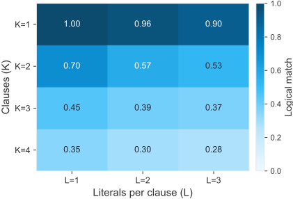
We evaluate rule recovery on synthetic DNF formulas with varying clause count K ∈ {1, 2, 3, 4} and literals per clause L ∈ {1, 2, 3}, testing at N=12 features (in-distribution, matching training range N ∈ [6, 12]). For each (K,L) configuration, we generate 200 random DNF rules per seed across 10 seeds and measure logical equivalence between the predicted and ground-truth rules.
Figure 2 shows that recovery degrades with complexity along both dimensions. For the simplest rules (K=1, L=1), logical match reaches 99.5%. This drops to 91.5% at L=2 and 81.7% at L=3. Increasing clause count has a larger effect: at K=4, L=1, recovery falls to 34.2%, and the most complex rules (K=4, L=3) achieve 24.0% logical match. Prediction accuracy remains high (85-100%) even when logical match is lower. The clause dimension (K) dominates difficulty because multi-clause rules require discovering multiple independent patterns, while longer clauses (L) only demand more precise literal selection within a single pattern.
5.3 Label Noise Robustness
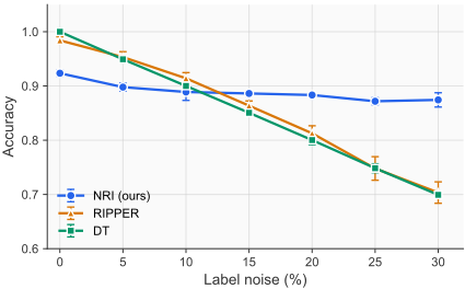
We evaluate robustness to label noise (random flips) against two interpretable baselines, RIPPER and DT. Figure 3 shows NRI accuracy stays stable (92.3%→87.4% at 30% noise), while RIPPER and DT degrade sharply (98.4%→70.3% and 100%→69.9% respectively). Symbolic methods are more accurate at low noise by fitting training data exactly, but beyond 15% noise NRI's statistical encoding provides implicit regularization and outperforms both baselines by 17 percentage points at 30% noise.
5.4 Spurious Variable Robustness
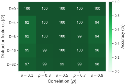
We test whether NRI ignores spurious features that correlate with labels but are not in the true rule. We append D ∈ {0, 4, 8, 16, 32} distractors per episode with P (d=1|Y =1) = ρ and P(d=1|Y=0) = 1-ρ for ρ ∈ {0.1, . . . , 0.9}, statistically predictive but causally irrelevant features. Figure 4 shows accuracy remains above 92% across all settings (97.6% at D=32, ρ=0.9; 96.7% at D=32, ρ=0.1 as the model learns to ignore the noise).
| Dataset | N | XGB | LGBM | EBM | RIPPER | RuleFit | FIGS | DT | N-DNF | NRI† | Gap |
|---|---|---|---|---|---|---|---|---|---|---|---|
| adult | 105 | 82.2 ± 0.2 | 82.7 ± 0.2 | 83.8 ± 0.1 | 81.9 ± 0.3 | 82.6 ± 0.2 | 82.8 ± 0.2 | 82.1 ± 0.2 | 83.0 ± 0.1 | 69.6 ± 4.4 | -14.2 |
| breast-cancer | 9 | 92.0 ± 1.4 | 65.5 ± 0.0 | 93.0 ± 1.2 | 88.3 ± 1.4 | 90.8 ± 2.2 | 89.6 ± 2.3 | 89.3 ± 2.6 | 90.3 ± 1.3 | 88.3 ± 0.3 | -4.7 |
| car | 21 | 80.5 ± 1.1 | 75.0 ± 1.6 | 81.2 ± 0.3 | 90.3 ± 0.9 | 94.2 ± 0.6 | 91.8 ± 1.3 | 78.7 ± 1.3 | 93.3 ± 1.0 | 51.2 ± 5.4 | -43.0 |
| credit | 46 | 82.1 ± 1.4 | 55.5 ± 0.0 | 82.2 ± 1.6 | 83.1 ± 2.1 | 81.7 ± 1.8 | 81.2 ± 1.7 | 81.3 ± 1.7 | 81.4 ± 2.6 | 71.5 ± 7.3 | -11.6 |
| diabetes | 8 | 67.4 ± 2.6 | 65.1 ± 0.0 | 66.9 ± 1.8 | 66.8 ± 2.2 | 65.5 ± 1.9 | 64.9 ± 2.0 | 65.3 ± 1.6 | 64.4 ± 2.3 | 68.0 ± 2.4 | +0.0 |
| german | 61 | 66.9 ± 1.1 | 70.0 ± 0.0 | 68.1 ± 1.7 | 58.3 ± 3.2 | 65.8 ± 1.0 | 64.6 ± 2.0 | 64.6 ± 2.4 | 68.1 ± 1.4 | 59.8 ± 3.8 | -10.2 |
| hepatitis | 32 | 79.4 ± 0.0 | 79.4 ± 0.0 | 81.2 ± 2.0 | 20.6 ± 0.0 | 20.6 ± 0.0 | 72.1 ± 3.2 | 73.8 ± 4.3 | 68.5 ± 5.3 | 55.9 ± 3.7 | -25.3 |
| ionosphere | 34 | 66.3 ± 4.3 | 64.1 ± 0.0 | 69.1 ± 3.9 | 59.5 ± 3.3 | 69.2 ± 6.0 | 63.8 ± 6.3 | 65.4 ± 5.1 | 67.8 ± 4.5 | 62.8 ± 3.9 | -6.4 |
| kr-vs-kp | 73 | 93.2 ± 0.6 | 90.7 ± 1.9 | 92.5 ± 0.5 | 89.9 ± 1.2 | 93.8 ± 0.7 | 92.7 ± 0.8 | 92.4 ± 0.6 | 92.0 ± 0.8 | 72.3 ± 5.3 | -21.5 |
| mushroom | 116 | 99.0 ± 0.2 | 99.1 ± 0.2 | 99.4 ± 0.1 | 98.5 ± 0.4 | 99.5 ± 0.2 | 99.4 ± 0.2 | 99.3 ± 0.2 | 98.8 ± 0.3 | 87.8 ± 3.9 | -11.7 |
| nursery | 27 | 90.5 ± 0.5 | 91.2 ± 0.4 | 91.1 ± 0.7 | 86.2 ± 1.0 | 88.5 ± 0.8 | 87.1 ± 0.5 | 84.8 ± 0.7 | 86.6 ± 0.7 | 71.3 ± 4.3 | -19.9 |
| spambase | 57 | 89.7 ± 0.6 | 89.8 ± 0.4 | 91.1 ± 0.6 | 85.7 ± 1.2 | 89.8 ± 0.4 | 85.7 ± 0.7 | 85.0 ± 1.0 | 87.8 ± 0.7 | 71.9 ± 0.7 | -19.2 |
| tic-tac-toe | 27 | 69.4 ± 2.6 | 65.3 ± 0.0 | 70.2 ± 1.2 | 56.0 ± 4.4 | 65.7 ± 1.5 | 64.8 ± 2.0 | 64.8 ± 1.3 | 67.8 ± 2.7 | 56.6 ± 2.5 | -13.6 |
| vote | 32 | 92.9 ± 1.8 | 61.4 ± 0.0 | 87.4 ± 2.1 | 91.6 ± 2.2 | 91.1 ± 1.6 | 90.5 ± 1.7 | 90.7 ± 2.4 | 91.8 ± 1.6 | 88.3 ± 1.8 | -4.6 |
| Mean | 82.2 ± 11.2 | 75.4 ± 13.5 | 82.7 ± 10.6 | 75.5 ± 21.0 | 78.5 ± 20.4 | 80.8 ± 12.4 | 79.8 ± 11.5 | 81.6 ± 11.8 | 69.7 ± 12.0 | -13.0 |
| Ablation | UCI Accuracy (%) | ∆Acc | Avg Clauses | Avg Literals |
|---|---|---|---|---|
| Full (baseline) | 74.8 ± 3.8 | - | 7.3 ± 1.2 | 3.2 ± 0.2 |
| - CF Necessity | 74.1 ± 4.7 | -0.6 | 7.8 ± 0.5 | 3.1 ± 0.3 |
| - Max-Margin | 72.0 ± 2.4 | -2.8 | 7.7 ± 0.4 | 3.2 ± 0.2 |
| - Slot Balance | 73.3 ± 3.7 | -1.5 | 7.0 ± 1.5 | 3.0 ± 0.5 |
5.5 Computational Scaling
We measure inference time and memory as problem size (N) and example count (M) vary. Latency stays nearly constant (∼7.5ms) as M grows from 32 to 512, and increases sublinearly with N (4.2ms→11.8ms for a 32× increase from N=16 to N=512); memory scales O(N 2 ) due to attention. At N=512, inference completes in under 12ms with 593MB peak memory. Full curves are in Appendix D.
5.6 Loss Ablation Study
Each loss contributes (Table 2): removing CF Necessity, Max-Margin Coverage, or Slot Balance drops UCI accuracy by 0.7%, 2.8%, and 1.5% respectively, with characteristic failure modes (more spurious-literal selection, unstable gate entropy, clause monopoly with slot variance jumping from 0.003 to 0.35). Rule complexity (7-8 clauses, 3 literals) is similar across ablations, so these losses primarily affect which literals are selected. The full model achieves the highest accuracy (74.8%) while maintaining interpretable rule sizes.
6 Conclusion
We presented Neural Rule Inducer (NRI), a foundation model for zero-shot rule induction trained entirely on synthetic Boolean formulas. By encoding literals through identityfree statistical properties (class-conditional rates, entropy, cooccurrence) and synthesizing clauses with a parallel slotbased decoder under product T-norm semantics, NRI is trained end-to-end on prediction accuracy alone and induces interpretable DNF rules on new domains without retraining. We believe this work opens up the possibility of foundation models for symbolic reasoning. Future work extends to multi-valued and continuous variables and to first-order logic with relational predicates.
Acknowledgements
This work was supported by JSPS KAKENHI Grant Number 25K21269. This study was carried out using the TSUBAME4.0 supercomputer at Institute of Science Tokyo. The author also thanks Professor Katsumi Inoue for a helpful discussion on this research.
@inproceedings{ijcai2026p445,
  title     = {A Foundation Model for Zero-Shot Logical Rule Induction},
  author    = {Phua, Yin Jun},
  booktitle = {Proceedings of the Thirty-Fifth International Joint Conference on
               Artificial Intelligence, {IJCAI-26}},
  publisher = {International Joint Conferences on Artificial Intelligence Organization},
  editor    = {Diego Calvanese},
  pages     = {3999--4007},
  year      = {2026},
  month     = {8},
  note      = {Main Track},
  doi       = {10.24963/ijcai.2026/445},
  url       = {https://doi.org/10.24963/ijcai.2026/445},
}
TY - CPAPER TI - A Foundation Model for Zero-Shot Logical Rule Induction AU - Phua, Yin Jun T2 - Proceedings of the Thirty-Fifth International Joint Conference on Artificial Intelligence, IJCAI-26 PB - International Joint Conferences on Artificial Intelligence Organization PY - 2026 SP - 3999 EP - 4007 DO - 10.24963/ijcai.2026/445 UR - https://doi.org/10.24963/ijcai.2026/445 ER -Copied
Machine-readable versions of this paper, for tools and AI agents:





