Optimal LTLf Synthesis

1 Introduction

Strategy synthesis is a key problem in Artificial Intelligence (AI), where an autonomous agent must compute a strategy/policy/controller that guarantees task achievement despite uncertainty and nondeterminism in the environment [Reiter, 2001; Ghallab et al., 2016]. Automated synthesis from high-level temporal specifications addresses this challenge by allowing designers to describe what the agent should achieve, while the synthesis process determines how to do so. This is formalised by reactive synthesis [Pnueli and Rosner, 1989], where the agent interacts with an adversarial environment and must ensure satisfaction of the specification under all possible environment behaviours.

For finite and terminating tasks, Linear Temporal Logic over finite traces (LTLf ) [De Giacomo and Vardi, 2013] provides a natural specification language, and LTLf synthesis [De Giacomo and Vardi, 2015] constructs strategies that guarantee satisfaction of an LTLf formula along every possible execution. LTLf synthesis shares deep similarities with planning in fully observable nondeterministic domains (FOND, strong plans) [Cimatti et al., 2003; Geffner and Bonet, 2013].

Standard approaches to LTLf synthesis [Pnueli and Rosner, 1989; De Giacomo and Vardi, 2015; Zhu et al., 2017; De Giacomo and Rubin, 2018] assume that an agent must satisfy a single LTLf formula while interacting with a fully adversarial environment [Aminof et al., 2019; Camacho et al., 2019]. Under this assumption, synthesis is typically an all-or-nothing approach: either a strategy that guarantees satisfaction of the specification exists, or the specification is declared unrealisable and no strategy is returned. While this model offers strong correctness guarantees, it is often too restrictive in practice, since real environments are rarely fully adversarial [Aminof et al., 2021; Ghallab et al., 2016] and users may struggle to capture all desired objectives in a single specification [Dimitrova et al., 2020; De Giacomo et al., 2025].

To overcome these limitations, prior work has mainly explored two directions. One direction extends the specification formalism to allow multiple objectives, as in preferencesbased planning, such as planning with soft goals [Son and Pontelli, 2006; Bienvenu et al., 2006; Jorge and McIlraith, 2008; Keyder and Geffner, 2009] and maximum realisability for temporal logic specifications [Dimitrova et al., 2020], which focuses on safety properties treated as soft constraints and allows their temporary violation. Another direction relaxes assumptions about the environment: best-effort synthesis [Aminof et al., 2021; De Giacomo et al., 2025] or strong cyclic planning [Cimatti et al., 2003; Geffner and Bonet, 2013], for example, allow agents to exploit cooperative environment behaviours instead of giving up when strict guarantees cannot be enforced.

In this paper, we focus on LTLf synthesis with multiple objectives and study the problem of optimal synthesis, especially when the conjunction of all objectives is not realisable. Here, the synthesis problem is no longer whether a strategy that guarantees all specifications exists, but to find a strategy that guarantees as many of the specifications as possible.

But what makes a strategy optimal? That depends on the circumstances. Consider an agent where we have five goals of equal value, e.g. that a robot eventually visits Rooms 1 through 5. The robot first chooses either a path that allows it to surely visit Room 1, or to go down a path where, depending on a choice of the environment, it can guarantee either to visit Rooms 2 and 3 or to visit Rooms 4 and 5.

If we only value guarantees that we can give a priori, then we would favour being sure to visit Room 1. We refer to this as max-guarantee synthesis: max-guarantee synthesis provides the maximal (or maximally valued) subset of objectives that can be jointly realised in the classic sense.

If we want to maximise (the value of) the specifications that we will achieve, on the other hand, we would prefer to satisfy two goals, even if we cannot commit to any of them in particular. We introduce max-observation synthesis to address this problem. Instead of committing to a fixed subset of objectives in advance, max-observation synthesis evaluates a strategy based on the objectives it actually satisfies along each execution, and focuses on maximising the number (or value) of achieved objectives.

In the robot example, we would steer the robot towards the point where it can ensure visiting two rooms, albeit which ones is down to the environment. This strategy exploits observed environment behaviour, making max-observation synthesis always at least as good as max-guarantee synthesis. Moreover, our framework naturally supports quantitative weights on objectives, enabling users to express the relative importance of individual objectives and allowing the synthesis of strategies that optimise the total achieved value.

We further improve max-observation synthesis to incremental max-observation synthesis, where we want to maximise the ensured number (value) of objectives for every history. In the robot example, the robot might find itself in a situation where, after visiting Room 2, it can choose to continue to Room 3, or go down a route where it can visit Rooms 4 and 5. If we only consider what the strategy can ensure from the beginning of its execution, these routes are of equal value, because other runs of the robot curtail this value to 2. In incremental max-observation synthesis, we want more: after each observed history, we seek a strategy that maximises the value that can be ensured from that point onward. In this setting, we would prefer visiting Rooms 4 and 5 over visiting Room 3 only, since-for the given history-this allows us to increase our promise to visit at least three rooms overall.

Both optimisation goals, max-guarantee and maxobservation, are natural and have their place: some goals are only worth satisfying if one can guarantee them a priori, while in other cases it is just as good to see them satisfied a posteriori. We thus study both and show that they can be combined.

We have implemented optimal LTLf synthesis using symbolic techniques [Zhu et al., 2017; Duret-Lutz et al., 2025], including max-guarantee synthesis, max-observation synthesis, and incremental max-observation synthesis. We also evaluated these approaches on benchmarks taken from the LTLf synthesis track of the annual reactive synthesis competition SyntCOMP (available at https://www.syntcomp.org/), for which we have constructed our own multi-objective specifications. Our empirical results show that the different approaches exhibit broadly comparable performance and solve a large fraction of the benchmarks, producing more informative strategies than simply concluding "unrealisable". Incremental max-observation synthesis shows similar, sometimes better, performance than non-incremental max-observation, demonstrating that strictly better guarantees can be obtained in practice at little additional cost. 1

2 Preliminaries

A trace over an alphabet of symbols Σ is a finite or infinite sequence of elements from Σ. The empty trace is ϵ. Traces are indexed starting at zero, and we write π = π0π1 · · · . The length of a trace is |π|. For a finite trace π, we denote by lst(π) the index of the last element of π, i.e. |π| - 1. For i ≤ lst(π), we have that πi ∈ 2AP is the i-th interpretation of π. By πk = π0 · · · πk we denote the prefix of π up to the k-th iteration.

2.1 LTLf Basics

Linear Temporal Logic on finite traces (LTLf ) is a specification language to express temporal properties for finite nonempty traces [De Giacomo and Vardi, 2013]. LTLf shares the syntax with LTL [Pnueli, 1977]. Given a set of atoms AP , the LTLf formulas over AP are generated as follows:

p ∈ AP is an atom, X! (Next), and U (Until) are temporal operators. We use standard Boolean abbreviations such as ∨ (or) and ⊃ (implies), tt (true) and ff (false). Moreover, we define the following abbreviations: Weak Next Xφ ≡ ¬X!¬φ, Eventually Fφ ≡ tt Uφ and Always Gφ ≡ ¬F¬φ. The size of φ, written |φ|, is the number of its subformulas. We assume standard semantics from [De Giacomo and Vardi, 2013].

An LTLf formula φ can be represented by a Deterministic Finite Automaton (DFA) Aφ = (2AP , Q, q0, δ, F ), where 2AP is a finite alphabet, Q is a finite set of states, q0 ∈ Q is the initial state, δ : Q× 2AP →Q is the transition function, and F ⊆ Q is the set of accepting states, such that, for every trace π, we have π |= φ iff π is accepted by Aφ [De Giacomo and Vardi, 2013].

2.2 LTLf Synthesis

An LTLf synthesis specification can be described by a tuple (φ, X , Y), where φ is an LTLf formula over the propositions in X ∪Y. X and Y are two disjoint sets: X is the set of input variables controlled by the environment and Y is the set of output variables controlled by the agent. A strategy is a function σ : (2X )∗ → 2Y that maps each finite sequence of input variables to an output assignment. X ∈ (2X )ω denotes an infinite sequence of valuations of input variables, and the trace π(X, σ) induced by the prefix of X and σ is:

Definition 1 (Winning strategy). Given an LTLf synthesis specification (φ, X , Y), a strategy σ : (2X )∗ → 2Y is a winning strategy for φ, denoted σ ▷ φ, if for every infinite sequence of the input variables X ∈ (2X )ω , the induced trace π(X, σ) satisfies φ, i.e. there exists a finite prefix of π(X, σ) that satisfies φ.

1 The full version of this paper: https://arxiv.org/abs/2605.11544

Definition 2 (Realisability). An LTLf synthesis specification (φ,X, Y) is realisable if there exists a winning strategy σ : (2X )∗ → 2Y for φ, i.e. σ ▷φ. The LTLf realisability problem is to determine whether (φ, X , Y) is realisable.

Definition 3 (Synthesis). The synthesis problem consists in computing a winning strategy for a realisable specification.

Sometimes, for simplicity, we omit X and Y when they are clear from the context.

2.3 DFAGames

Classic solutions to LTLf synthesis rely on a reduction to two-player DFA games (reachability games). A DFA game is described as a tuple G = (A, F), where A = (2AP ,Q, q0, δ,-) is a DFA representing the game arena of which the set of accepting states does not matter and F ⊆ Q is the reachability winning objective. For LTLf synthesis, we often take the corresponding DFA of the formula as the game arena and the set of accepting states as the winning objective. Given a play π = (X0 ∪ Y0)(X1 ∪ Y1) . . . ∈ (2X∪Y )ω , running A on π gives us the infinite sequence ρ = q0q1 . . . ∈ Qω such that q0 is the initial state and qi+1 = δ(qi,Xi ∪ Yi) for all i ≥ 0. Since the transitions in A are all deterministic, we thus denote by ρ = run(π,A) the unique sequence of running A on π. Analogously, we denote by ρk = run(πk ,A) the unique finite sequence of running πk on A, and ρk = q0q1 . . . qk. The reachability winning objective F indicates a set of desired states to reach for the agent. A play π is a winning play with respect to winning objective F if some state s ∈ F occurs in run(π,A). An agent strategy σ is winning in G = (A, F) if for every infinite sequence of the input variables X ∈ (2X )ω , the induced play π(X, σ) is a winning play with respect to F.

A DFA game with reachability objective G = (A, F) can be solved by the following least fixed point computation.

where PreC(S) = {q ∈ Q | ∃Y ∈ 2Y .∀X ∈ 2X .δ(q, (X, Y )) ∈ S} is the controllable preimage. The computation stabilises at the least index i such that Wini+1(G) = Wini(G) and we denote this fixed point by Win(G) = Wini(G). Every state q ∈ Win(G) is a winning state for the agent, from where she has a winning strategy in the game Gq = (Aq, F), where Aq = (2X∪Y ,Q, q, δ,-), i.e. the same arena A but with the new initial state q. Intuitively, Win(G) represents the "agent winning region", from which the agent is able to win the game, no matter how the environment behaves.

3 Optimal Synthesis

We consider a set Φ of LTLf formulas, of which we intuitively want to satisfy as many as possible. Φ is realisable (resp. unrealisable) if ∧φ∈Φ φ is realisable (resp. unrealisable), i.e. there exists (resp. does not exist) a winning strategy for Φ. The case we are interested in is where Φ is unrealisable, but we can realise as large, or important, a subset of Φ as possible. When posing this question, we have to define whether this means first selecting the subset Ψ ⊆ Φ we promise to realise and then executing the agent with the goal of realising Ψ (guarantee synthesis), or if we find a strategy whose traces satisfy potentially different subsets Ψ1, . . . ,Ψn ⊆ Φ of Φ, and we maximise the minimal value of the trace (observation synthesis). We consider both versions as well as a combination, where we maximise a weighted sum of the two values.

Let Φ be a set of LTLf formulas over the alphabet 2X∪Y , where X and Y are a fixed partition of the atoms into environment input and agent output, respectively. Let P = (Φ, X , Y) be a tuple and G, V : Φ → (0, 1] be functions specifying the preference value of every LTLf formula φ ∈ Φ as guarantee (G) and observed value (V ), respectively.

We first define the max-guarantee LTLf synthesis problem. Abusing the notation slightly, for a strategy σ : (2X )∗ → 2Y , we define the guarantee value of σ with respect to P as

Definition 4 (Max-guarantee winning strategy). Given P = (Φ, X, Y) and a guarantee value function G, a strategy σ∗ : (2X )∗ → 2Y is a max-guarantee winning strategy for P if

Definition 5 (Max-guarantee LTLf synthesis). Given P = (Φ,X, Y) and a guarantee value function G, the maxguarantee synthesis problem is to compute a pair (σ⋆ , v⋆ ), where σ⋆ : (2X )∗ → 2Y is a strategy and v⋆ ∈ R is its guarantee value, such that

Next, we define the max-observation LTLf synthesis problem. For a trace π : (2X∪Y )ω , we define the observed value of π with respect to P as

and the observed value of a strategy σ as

Definition 6 (Max-observation winning strategy). Given P = (Φ,X, Y) and an observed value function V , a strategy σ∗ : (2X )∗ → 2Y is a max-observation winning strategy for P if

Definition 7 (Max-observation LTLf synthesis). Given P = (Φ,X, Y) and an observed value function V , the maxobservation synthesis problem is to compute a pair (σ⋆ , v⋆ ), where σ⋆ : (2X )∗ → 2Y is a strategy and v⋆ ∈ R is its observed value, such that

All of these problems are in the same complexity class as ordinary LTLf synthesis.

Theorem 1. The max-guarantee and max-observation LTLf synthesis problems are 2EXPTIME-complete.

4 Max-Guarantee Synthesis

We now present a solution to the max-guarantee synthesis problem for an instance P = (Φ,X, Y) with a guarantee value function G. We show that the problem can be reduced to computing a strategy that realises a maximal subset of formulas, termed a max realisable core, such that every play induced by the strategy satisfies all formulas in this subset.

Definition 8 (Realisable core). Let Φ = {φ1, φ2, · · · , φn} be a set of LTLf formulas and Ψ ⊆ Φ a realisable subset of Φ. Ψ is a realisable core if for every φi ∈ Φ\Ψ, φi ∧ ∧φj∈Ψ φj is unrealisable.

Definition 9 (Max realisable core). A realisable core Ψ∗ ⊆ Φ is maximal if for any other realisable core Ψ′ ⊆ Φ, it holds that ∑φ∈Ψ∗ G(φ) ≥ ∑φ∈Ψ′ G(φ).

It is straightforward to see that the max-guarantee synthesis problem, computing the maximal guarantee v∗ , can be reduced to computing a maximal realisable core Ψ∗ , where v∗ = ∑φ∈Ψ∗ G(φ). We solve the max-guarantee synthesis problem in the following steps:

• Step 1: Automata Construction. For every LTLf formula φi ∈ Φ, we build its corresponding DFA Ai = (2X∪Y , Qi , qi0 , δi , F i ), where F i ⊆ Qi is the set of accepting states for φi.

Step 2: Game Arena Construction. We build the product automaton A = ⊗φi∈Φ Ai , such that A = (2X∪Y , Q, q0, δ, ∅), where Q = ×φi∈ΦQi is the product state space, q0 = (qi0 )φi∈Φ is the initial state, δ is the product transition function induced by the {δi }φi∈Φ.

Step 3: Guarantee Value-Based Partition. We partition the search space into a sequence of formula subsets ordered by non-increasing guarantee values. For each φi ∈ Φ, we define F i⊗ = {(q1, · · · , qn) ∈ Q | qi ∈ F i } as the set of states in the product automaton where φi is among the satisfied specifications. We then consider the finite set of values v1 > v2 > · · · > vℓ such that each vj = ∑φ∈Ψ G(φ) can take for subsets Ψ of Φ, and define FΨ = ⋂φi∈Ψ F i⊗.

Step 4: Game Solving. We iterate over the value v from Step 3 in non-increasing order. For each Ψ, we construct the DFA game GΨ = (A, FΨ), using the product automaton A from Step 2 as the game arena and FΨ as the set of accepting states. Then we solve the game GΨ by computing its winning set Win(GΨ). The max-value v∗ is the first v that satisfies q0 ∈ Win(GΨ); we return a winning strategy of GΨ where Ψ is a max realisable core.

The overall synthesis procedure is presented in Algorithm 1. The algorithm iterates through FΨ in non-increasing order of guaranteed values (Lines 2-4) to ensure that the first realisable core found is maximal. Once a realisable core Ψ is found via the reachability check (Lines 7-8), the corresponding guaranteed value with a winning strategy is returned.

The correctness of Algorithm 1 is ensured by the guaranteed value-based non-increasing search strategy.

Theorem 2. Algorithm 1 returns a max-guarantee v = ∑φ∈Ψ G(φ) where Ψ is a max realisable core. That is, the Algorithm 1 Max-Guarantee Synthesis

Require: A set of LTLf formulas Φ = {φ1, · · · , φn} Ensure: A winning strategy σ∗ for a max realisable core Ψ ⊆ Φ, and ∑φ∈Ψ G(φ)

• 1: Construct the product automaton A fromΦ
• 2: Partition the search space into a sequence of subsets S = (Ψ1,Ψ2, . . . ,Ψ2|Φ|) where ∑φ∈Ψi G(φ) ≥ ∑φ∈Ψi+1 G(φ) holds for all i < 2|Φ| .
• 3: for j in 1 to 2|Φ| do
• 4: FΨj ← ⋂φi∈Ψj F i⊗
• 5: Construct DFA game GΨj = (A, FΨj )
• 6: Compute winning set Win(GΨj ) and extract a winning strategy σ∗
• 7: if q0 ∈ Win(GΨj ) then
• 8: return (σ∗ , ∑φ∈Ψj G(φ))
• 9: end if
• 10: end for

subset Ψ is realisable, and for any other realisable subset Ψ′ ⊆ Φ, it holds that ∑φ∈Ψ G(φ) ≥ ∑φ∈Ψ′ G(φ).

Theorem 3. The running time of Algorithm 1 is O(2|Φ| · |A|), where |A| is the size of the product automaton A.

We note that we build the arenas ⊗φi∈Ψ Ai individually for each Ψ. Normally, the structures of the Ai are such that these automata are substantially smaller than A for Ψ ̸= Φ. In this case the running time for Ψ = Φ normally dominates.

5 Max-Observation Synthesis

In this section, we first present a basic algorithm for computing a strategy for max-observation synthesis. We then introduce incremental max-observation synthesis, where the synthesis space is updated dynamically with the execution history trace, and show how to adapt the basic algorithm to construct an incremental max-observation strategy, followed by an improved algorithm.

5.1 Basic Algorithm

The basic algorithm for the max-observation synthesis problem begins with automata construction and game arena construction, which coincide with the first two steps of the maxguarantee synthesis procedure described in Section 4. We describe the remaining steps as follows:

Step 3: Target Construction. For each φi ∈ Φ, we define F i⊗ = {(q1, · · · , qn) ∈ Q | qi ∈ F i } as the set of states in the product automaton where φi is among the satisfied specifications. We then consider the finite set of values v1 > v2 > · · · > vℓ that ∑φ∈Ψ V (φ) can take for subsets Ψ of Φ, and define Fv = ⋃{FΨ | ∑φ∈Ψ V (φ) ≥ v} for each of these values, where FΨ = ⋂φi∈Ψ F i⊗.

Step 4: Game Solving. We iterate over the value v from Step 3 in descending order. We construct the DFA game Gv = (A, Fv), using the product automaton A from Step 2 as the game arena and Fv as the reachability winning objective. Then we solve the game Gv by computing its winning set Win(Gv). The max-value v∗ is the first v that satisfies q0 ∈ Win(Gv); we return a winning strategy of Gv∗ .

The following lemma is key to the correctness of the basic algorithm of the max-observation synthesis problem.

Lemma 4. Let P = (Φ, X , Y) with the observed value function V be a max-observation synthesis problem and Win(Gv) the agent winning region of the reachability game Gv = (A, Fv), computed as above, where v is an arbitrary value. Then there is a strategy σ with ensured value v, i.e. V (σ) ≥ v iff q0 ∈ Win(Gv).

Theorem 5. Let P = (Φ,X, Y) with the observed value function V be a max-observation LTLf synthesis problem and v∗ the first value (in descending order) such that q0 ∈ Win(Gv∗), where Gv∗ = (A, Fv∗). Let σ∗ be any winning strategy for Gv∗ returned by Step 4. Then σ∗ is a maxobservation winning strategy for P, and the maximal realisable value is v∗ (i.e. V (σ∗ ) = v∗ ).

We conclude by showing that the complexity of the basic algorithmmatches that of the max-observation LTLf synthesis problem.

Theorem 6. The running time of the basic algorithm is O(2|Φ| · |A|), where |A| is the size of the product automaton A.

We note that this can be improved to O(|Φ| · |A|) (or: O(ln(ℓ) · |A|)) by considering the values along an ordered tree: if there are f > 1 feasible values left, we can next test for the f/2 largest among them (rounded up or down), reducing the feasible values to ⌈f/2⌉ and providing ln(ℓ) iterations (e.g. O(ln(|Φ|)) if all formulas have the same value).

The above basic algorithm solves the max-observation synthesis problem. We extend this algorithm in the next subsection by introducing the concept of incremental maxobservation synthesis, where the synthesis space is updated dynamically with the execution history trace.

5.2 Incremental Max-Observation Synthesis

The goal of the principled algorithm from the previous section is to provide maximal ensured value. However, after a prefix h ∈ (2AP )∗ , we might be in a position to provide better ensured values. We first define the set of prefixes of a strategy σ, denoted pre(σ) ⊆ (2AP )∗ , the set of prefixes of {π(X, σ) | X ∈ (2X )ω } of runs induced by σ. Conversely, we define strategies compatible with a history h ∈ (2AP )∗ as comp(h) = {σ ∈ (2X )∗ → 2Y | h ∈ pre(σ)}. Then for all h ∈ pre(σ), we define

Definition 10 (Incremental max-observation optimal strategy). Given P = (Φ, X , Y) with an observed value function V , a strategy σ∗ : (2X )∗ → 2Y is observation optimal for a history h ∈ pre(σ∗ ) for P if

holds, and incremental observation optimal if it is observation optimal for all histories h ∈ pre(σ) for P.

Extending the Basic Algorithm. To synthesise an incremental observationally optimal strategy, we can adapt the basic algorithm from Section 5.1. In particular, in Step 4, after solving each DFA game Gv, we record for every game state q the maximal value vq such that q ∈ Win(Gvq ), together with the corresponding local strategy σq ∈ 2Y . This local strategy can be viewed as the first move of an optimal strategy for the game Gvq when the initial game state is replaced by q. Finally, we combine the local strategies σq for all game states q into a global strategy σ: (2X )∗ → 2Y and show that σ is an incremental observationally optimal strategy.

The correctness of this procedure follows from the fact that whenever a game state q of the product automaton A is reached under the strategy σ, it follows the corresponding local strategy σq, thus achieving the maximal observed value vq when q is treated as the initial state of the game.

Improved Algorithm. While the basic algorithm can be adapted to compute an incremental max-observation optimal strategy, it is theoretically inefficient, as each game state and state-action pair may be considered multiple times: a state q ∈ Win(Gvi ) also belongs to Win(Gvj ) for all j > i. To synthesise an incremental max-observation optimal strategy efficiently, we retain the first two steps of the algorithm and then perform incremental game solving and target construction directly.

Step 3: Incremental Max-Obs Optimal Strategy Computation. We set W0 = ∅ and then iteratively calculate targets of increasing size as follows for k = 1, . . . , ℓ:

• F = vk = ⋃{FΨ | ∑φ∈Ψ V (φ) = vk}
• Tk =Wk-1 ∪F = vk , Gk = (A, Tk), and Wk = Win(Gk) until q0 ∈ Wk.

We use the attractor strategies to each target Tk to define σ∗ (and fix it arbitrarily elsewhere).

The correctness of the improved algorithm is based on two facts: (1) Wk = Win(Gvk ) where Gvk = (A, Fvk ) is the DFA game constructed in Step 4 of Section 5.1; and (2) for any history h, if the maximal achievable value has not already been observed along h, then the state qh reached by h must belong to Win(Gv∗) to enforce v∗ .

Theorem 7. Let P = (Φ, X , Y) with an observed value function V be an incremental max-observation LTLf synthesis problem and vk∗ the first value (in descending order) such that q0 ∈ Win(Gk∗), and σ∗ be a strategy returned by our algorithm. Then σ∗ is incremental observation optimal.

While the improved algorithm works on the same arena as the algorithm described in the previous section, it never considers a state-action pair twice. When explicitly constructing the arena A, the sets F = vk can be built with it. In this case, each state is considered at most twice across all fixed point computations: once when added to one of the F = vk and once when added to a winning region during fixed point construction.

Theorem 8. The running time of the improved algorithm is O(|A|), where |A| is the size of the product automaton A.

This is in contrast to the principled algorithm from the previous section, where every state and state-action pair can be considered once per fixed point construction.

As an additional computational advantage, computing Win(Gk) could take fewer steps than computing Win(Gvk ) since we start with a larger target (Tk ⊇ Fvk ).

5.3 Combination withMax-Guarantee

It is straightforward to combine (incremental) maxobservation with max-guarantee: to compute the (incremental) max-observation value subject to guaranteeing a given subset Γ ⊆ Φ of Φ, we can simply define Fv,Γ = ⋃{FΨ | ∑φ∈Ψ V (φ) ≥ v, Ψ ⊇ Γ} and F = v,Γ = ⋃{FΨ | ∑φ∈Ψ V (φ) = v, Ψ ⊇ Γ}.

We can then find optimal solutions and values v∗Ψ for (incremental) max-observation for each Ψ ⊇ Γ individually for realisable Ψ (note that, for Ψ ̸= ∅, Ψ is realisable iff v∗Ψ > 0 holds, so that the realisability of Ψ is obtained as a side product and does not have to be tested individually), and find the best value v∗Ψ + ∑φ∈Ψ G(φ) for realisable Ψ.

6 Symbolic Optimal Synthesis

In this section, we introduce symbolic techniques of our proposed approaches to optimal LTLf synthesis. The symbolic techniques below are faithful encodings of the explicit constructions, following the symbolic framework of [Zhu et al., 2017]. Their correctness follows from Theorems 2, 5, and 7.

Symbolic DFAGames. We utilise the symbolic techniques in [Zhu et al., 2017], where the symbolic representation of a DFA A = (2AP , Q, q0, δ, -) is a tuple As = (X , Y, Z, I, η), where Z is a set of variables such that |Z| = ⌈log |Q|⌉, and every state q ∈ Q corresponds to an interpretation Z ∈ 2Z over Z. I is a Boolean formula satisfied only by the interpretation of the initial state q0. η : 2X × 2Y × 2Z → 2Z is a Boolean function representing the transition function such that η = ⟨ηz0 , · · · , ηzm ⟩, where ηz : 2X ×2Y ×2Z → {0, 1}. Accordingly, we denote the symbolic reachability game as Gs = (As, g), where g is a Boolean formula over Z representing the reachability objective.

The game can be solved by symbolic fixpoint computation over two Boolean formulas w over Z and t over Z∪Y, which represent the agent winning region and winning state-action pairs, respectively. The initial step is w0(Z) = g(Z) and t0(Z, Y) = g(Z). ti+1 and wi+1 are constructed as follows:

The computation terminates when I |= wi. Then, we can use ti+1 to compute a winning strategy through the mechanism of Boolean functional synthesis [Fried et al., 2016]. Details of each step can be found in [Zhu et al., 2017].

6.1 Symbolic Max-Guarantee Synthesis

The symbolic characterisation of max-guarantee synthesis from Section 4 is relatively straightforward. Given a set of LTLf objectives Φ = {φ1, · · · , φn}, for each φi we construct a symbolic DFA Ais = (X, Y,Z i , I i , ηi , gi ). The symbolic product automaton As = (X, Y,Z, I, η,-) can be constructed on the fly by taking Z = ⋃i Z i , I = ∧i I i , and defining the transition function as η(Z,X, Y) =

∧i ηi (Z i ,X, Y). Since each ηi = ⟨ηiz0 , · · · , ηizm ⟩ is represented as a vector of Boolean update formulas over the state variables in Z i , the transition function η of the product automaton can be obtained simply by collecting these update formulas. Then, max-guarantee synthesis reduces to solving a sequence of symbolic DFA games GΨ = (As, gΨ), where gΨ = ∧ψi∈Ψ gi following the guarantee value-based partition as in Step 4 of Section 4.

6.2 Symbolic Max-Observation Synthesis

We follow the same DFA construction and symbolic product automaton construction as in max-guarantee synthesis. For each value v, the reachability objective of the corresponding symbolic game is gv = ∨Ψ⊆Φ:∑φ∈Ψ V (φ)≥v ∧φi∈Ψ gi . We then solve a sequence of reachability games following the descending order of v as in Step 4 of Section 5.1.

Symbolic Incremental Max-Observation Synthesis. Extending the basic max-observation synthesis algorithm to obtain an incremental max-observation optimal strategy relies on recording and combining winning information across values. Note that solving each game Gv produces two Boolean formulas: wv(Z) encoding the winning region Win(Gv) and tv(Z, Y), encoding winning state-action pairs. Instead of explicitly associating each state q with its maximal achievable value, we collect the pairs (wv, tv) obtained in descending order of v and construct an incremental observationally optimal strategy by prioritising higher values. We start from the winning state-action pairs of the highest value v1 and iteratively add new winning state-action pairs from lower-value games only for states not already winning at a higher value, i.e. t = tv1 ∨ ∨1<k≤v∗(tvk ∧¬wvk-1 ). The resulting formula t thus compactly represents incremental max-observation optimal strategies, and we then can utilise Boolean functional synthesis to obtain a single strategy from t.

Symbolic improved incremental max-observation algorithm performs incremental game solving directly on growing target sets. Each target set Tk is represented by a Boolean formula gTk = wk-1 ∨ g= vk , where g= vk encodes the states in F = vk and wk-1 is the winning region computed at the previous iteration. Since tk now encode local strategies for all winning states wk, incremental max-observation optimal strategies can be obtained by simply combining the collected winning state-action pairs tk from all iterations as t = t1 ∨ ∨k>1 (tk ∧ ¬wk-1). Note that, although the construction of t is syntactically identical to that used in the extension of the basic max-observation algorithm, the underlying reason differs. In the extension, tvk ⊆ tvk+1 holds due to repeated solving on nested targets, whereas this inclusion does not hold in the improved algorithm, since each iteration already includes the previous winning region in its target. Therefore, the term (tk ∧¬wk-1) is necessary to discard vacuous tt agent actions introduced at the initial fixpoint step of game Gk. The final strategy σ∗ is then synthesised from t using Boolean functional synthesis.

7 Experimental Evaluation

Implementation. We implemented a prototype tool, called OPTLTLFSYNT, to evaluate our approaches. OPTLTLFSYNT

uses Spot [Duret-Lutz et al., 2025] for state-of-the-art LTLf - to-DFA translation, and relies on the CUDD 3.0.0 [Somenzi, 2016] BDD library for symbolic synthesis, including Boolean formula representation and manipulation.

Benchmarks. We evaluate our approach on benchmarks taken from the LTLf synthesis track of SyntCOMP (https://www. syntcomp.org/). We restrict our evaluation to instances that are unrealisable and conjunction-decomposable, i.e. specifications given as a conjunction of multiple individual LTLf formulas, since our goal is to synthesise strategies that satisfy as many individual specifications as possible. Therefore, we have 1145 benchmark instances, in total. The number of conjuncts per instance ranges from 2 to 50.

Experiment setup. All tests were run on a MacBook with an Apple M4 chip (10 physical cores, up to 4.41 GHz) and 16 GB of RAM. The timeout was set to 300 seconds.

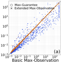
Evaluation results are shown in Figure 1. Generally, different methods work broadly equally fast, with a relatively small factor between them and different approaches perform faster on different instances. We have four approaches: max-guarantee, basic max-observation, extended max-observation, and improved max-observation (the latter two are for incremental max-observation synthesis). Within the 300s timeout, these approaches can solve 1060, 1005, 1006, 1008 instances, respectively, out of 1145 benchmarks with 30 instances timing out during individual LTLf -to-DFA construction, demonstrating the practical feasibility of our optimal LTLf synthesis techniques.

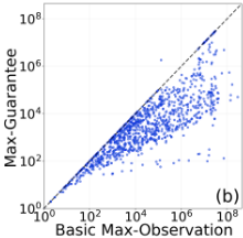
Specifically, max-observation achieves a strictly larger ensured value than that returned by max-guarantee synthesis on 16 instances. This confirms that optimising achieved value rather than a maximal realisable core can sometimes lead to realising more potential. As shown in Figure 1(a), maxguarantee is palpably faster than max-observation on a noticeable subset of instances. We believe that this is because subsets of specifications induce much smaller symbolic arenas due to the on-the-fly symbolic automata product. Maxobservation, on the other hand, has to always work on the full arena (but can generally realise more specifications and needs fewer calls), hence dealing with more complex game solving. Moreover, the target sets also become complex. In particular, timeouts occurred in cases where the target required satisfying, for example, 16 out of 20 objectives, which results in 4845 possible combinations. The corresponding target is a large disjunction of individual target sets, and the resulting BDDs (together with their successively constructed controlled attractors) can be large, making symbolic operations costly, as shown in Figure 1(b).

Figure 1(a) also shows that extending basic maxobservation to incremental strategies incurs only minor overhead, and in some cases even improves performance. This is again explained by the symbolic nature of the implementation, where strategy extraction relies on BDD-based Boolean functional synthesis. The iterative construction of t (see Section 6.2) can produce smaller and more structured BDD representations, which in turn accelerates strategy extraction.

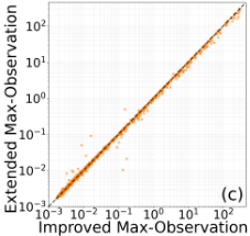
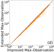
Figure 1(c) compares the extension of basic maxobservation with the improved max-observation algorithm. We can see that, despite solving slightly fewer instances, the extension can sometimes outperform the improved algorithm in runtime. This is, again, because the improved algorithm works on larger target sets in each game iteration, which can reduce the number of fixpoint iterations but makes each fixpoint (preimage) step more expensive in practice (see Figure 1(d)), despite its stronger theoretical guarantees.

The full version provides detailed experimental results.

8 Conclusions

We have studied optimal synthesis for LTLf specifications in cases where the conjunction of objectives is unrealisable. We introduced max-guarantee, max-observation, and incremental max-observation synthesis to capture different optimisation goals and to allow strategies to exploit the observed behaviour of the environment instead of always assuming a purely adversarial one. Our experimental evaluation on a prototype implementation shows that optimal LTLf synthesis has practical potential, with good scalability and only minor overhead. This work is a first step towards addressing unrealisability in LTLf synthesis. For future work, we plan to investigate on-the-fly techniques to further improve efficiency and extensions to synthesis under partial observability.

Acknowledgements

This work was supported by the EPSRC through the projects TRUSTED (EP/X03688X/1) and Games for Good (EP/X042596/1).