Social Welfare Under Heterogeneous Time Preferences

1 Introduction

Markov decision processes (MDPs) are canonical models of decision-making under uncertainty and form the backbone of several mature and widely deployed technologies, including reinforcement learning [Sutton and Barto, 2018], optimal control [Puterman, 1994], and economics and game theory [Bas¸ar and Olsder, 1999; Filar and Vrieze, 1997]. In settings where a single decision-making agent acts on behalf of multiple principals, the preferences of each principal are encoded by a distinct reward function that quantifies the instantaneous utility they associate with each decision. This work addresses the problem of synthesising strategies for the agent that maximise a utilitarian notion of social welfare, defined as the aggregate discounted payoffs across all principals.

Time Preference and Discounting. As an agent interacts with a system, it accrues infinite sequences of rewards on behalf of multiple principals. These rewards are typically aggregated using geometric discounting to evaluate the overall utility of a strategy. The discount factor plays a dual role. First, it imposes a notion of effective finiteness on the expected trajectory length. Second, it endows the optimisation process with desirable mathematical properties, such as value contraction [Shapley, 1953]. The discount factor also admits a behavioural interpretation [Tasdighi Kalat et al., 2024; Tasdighi Kalat et al., 2026] rooted in human decision-making and captures the principle of time preference, namely that a dollar today is valued more than a dollar tomorrow.

Heterogeneous Time Preferences. Inmany real-world settings, principals do not share identical attitudes toward delayed rewards. While discounting is commonly used to aggregate long-run payoffs, the choice of discount factor reflects an underlying time preference and may vary across principals due to structural incentives, institutional roles, or strategic priorities. Consequently, assuming a common discount factor can be overly restrictive and may obscure natural asymmetries in how principals value future outcomes.

This motivates the study of MDPs in which multiple principals, each with their own reward function and discount factor, delegate decision-making to a single agent constrained to follow a common strategy. In such settings, the agent must reconcile heterogeneous time preferences when optimising behaviour. Our objective is to synthesise strategies that resolve this tension in service of the common good by maximising a utilitarian notion of social welfare, defined as the aggregate discounted payoff across all principals.

The Need for Memory. In the well-studied setting where all principals share the same discount factor, optimal strategies are known to be positional. In contrast, we show that memory becomes necessary to maximise social welfare even in simple settings involving only two principals who receive identical rewards at every decision point.

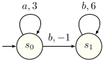
(a) Investment MDP shared by two principals: Alice, with α = 23 , and Bob, with β = 13 .

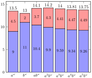
• (b) Discounted payoffs; stacked bars indicate social welfare. Blue: Alice, Red: Bob.

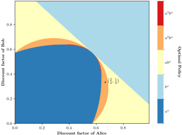
(c) Socially optimal waiting time over (α, β).

Figure 1: Heterogeneous discounting: the investment MDP, resulting payoffs across strategies, and the induced optimal waiting-time map.

Example 1 (Memory is necessary under heterogeneous discounting). Consider a scenario in which two principals, Alice and Bob, jointly operate a hotel and must decide whether to update and expand it. If they continue operating the hotel without investment (action a from state s0), they each earn $3 million per year. If they choose to update and expand (action b from s0), they incur a one-time cost of $1 million each and transition to state s1, where they earn $6 million annually thereafter; see Figure 1a. Although both principals receive the same rewards, they differ in their discount factors: Alice discounts the future at α = 2 3 , while Bob discounts more steeply at β = 13 .

The space of strategies consists of either remaining in s0 forever, denoted aω , or staying in s0 for k steps and then transitioning to s1, denoted ak bω . For each principal with discount factor λ ∈ {α, β}, the discounted payoff for the strategy aω is 3 1-λ . For the strategy ak bω , the payoff is:

If maximising Alice's payoff, the agent would invest and move to s1; in contrast, given Bob's steeper discounting, it would prefer remaining in s0 indefinitely. However, neither strategy maximises social welfare.

The optimal strategy remains in s0 for two steps before transitioning to s1, i.e., a2 bω . Although suboptimal for each principal individually, this compromise yields higher social welfare: Bob's gain from deferring the transition outweighs Alice's loss. Delaying beyond two steps, however, causes Alice's utility to decline faster than Bob's gain, reducing aggregate welfare. Figure 1b illustrates the resulting individual payoffs and social welfare across strategies.

The optimal number of steps to remain in s0 before transitioning to s1 depends on the specific discount factors of the two principals. Figure 1c shows how the socially optimal strategy varies over the space of discount factor pairs. Each region in the map corresponds to a fixed number of steps the agent must wait in s0 before executing the transition.

Contributions. We study a setting in which a single agent acts on behalf of multiple principals to optimise a utilitarian notion of social welfare, defined as the total discounted payoff accrued to all principals. The framework explicitly accommodates heterogeneous time preferences by allowing each principal to have an individual discount factor that contributes to the aggregated objective.

We first show that memoryless strategies are not sufficient for achieving optimal social welfare. Moreover, even when restricting attention to positional (memoryless) strategies, optimality may require randomisation. For example, in the hotel investment scenario (Example 1), a randomised positional strategy that selects action a in state s0 with probability 1/4 achieves an expected social welfare of 13.6, exceeding the welfare attained by any pure positional strategy.

We then study the computational complexity of optimising over such simpler strategy classes. We show that determining whether there exists a stationary pure or mixed strategy that achieves a given social-welfare threshold is NP-hard.

As our main contribution, we show that socially optimal strategies can always be chosen from a class of pure finitememory counting strategies. Furthermore, under mild spacing assumptions on the discount factors, namely that 1 α/β-1 is polynomially bounded in the input size for two discount factors α > β, as occurs when denominators are encoded in unary or discount factors are drawn from a finite set, such strategies can be synthesised efficiently, in polynomial time.

Finally, as a proof of concept, we implement our algorithm and demonstrate empirically that it scales well in practice.

A full version with omitted proofs, details, experiments, and examples is available on arXiv [Bahmani et al., 2026].

Related Work. Asymmetric discounting has been extensively studied in the context of repeated games, where it enables cooperative outcomes that are otherwise unsustainable under symmetric time preferences. Lehrer and Pauzner [1999] showed that heterogeneity in discount factors can expand the equilibrium payoff set, as more patient players are able to delay gratification to support cooperation-effectively subsidizing less patient players early on. Dasgupta and Ghosh [2022] further analysed how timepreference asymmetry reshapes incentives and enhances the stability of cooperative behaviour. These insights have been extended to multi-agent settings. In particular, Gu'eron et al. [2011] and Chen and Takashi [2012] show that in repeated games with heterogeneous discount factors, if all discount factors are sufficiently close to one, then any strictly individually rational payoff profile can arise as the outcome of a subgame-perfect equilibrium.

However, these works focus on stateless repeated games, where each round is structurally identical and independent of past actions, aside from discounting, and where players optimise only their own discounted payoffs. In contrast, our work introduces time-preference asymmetry into stateful stochastic games, where agents (acting on behalf of multiple principals) influence state transitions over time. In this setting, discounting interacts with system dynamics, leading to qualitatively new forms of strategic complexity. To the best of our knowledge, this is the first formal study of cooperative stochastic games with heterogeneous time preferences.

Our setting is fundamentally different from statedependent discounting in MDPs and stochastic games [Gan et al., 2023; Chatterjee et al., 2013]. There, discount factors may depend on the state, but are uniform across agents at each time step. Pitis [2023] adopts an axiomatic perspective and shows that aggregating objectives with different time preferences cannot be represented by a Markovian reward function. Their analysis considers multiple discount factors for the same agent. In contrast, we study a setting with multiple principals, each endowed with its own discount factor, and fix a utilitarian social-welfare objective. We then analyse the induced optimisation problem in stateful stochastic games.

Multi-objective optimisation is a related line of work, in which outcomes are evaluated with respect to multiple reward criteria and questions involve the synthesis of Pareto-optimal strategies or the comparison of outcomes under partial orders such as lexicographic preferences [Chatterjee et al., 2006; Chatterjee et al., 2013]. By contrast, the focus here is not on optimising multiple objectives, but on decision-making on behalf of multiple principals whose discounted utilities are aggregated into a utilitarian notion of social welfare.

2 Preliminaries

A probability distribution over a finite set S is a function d: S → [0, 1] such that ∑s∈S d(s) = 1. Let D(S) denote the set of all probability distributions over S.

Definition 1. AMarkov decision process (MDP)Mis a tuple (S,A, T), where S is a finite set of states, A a finite set of actions, and T : S ×A -⇁ D(S) is a transition function. For s ∈ S, let A(s) denote actions available at s. For s, s′ ∈ S and a ∈ A(s), we write p(s′ | s, a) to denote T(s, a)(s′ ).

We measure the size of Mby the size of its representation, where the values may be given in binary.

A run ρ of MDP M is an ω-word ⟨s0, a0, s1, a1, s2 . . .⟩ ∈ S × (A × S)ω such that p(sj+1|sj, aj) > 0 for all j ≥ 0. A finite run is a finite such sequence, that is, a word in S × (A × S)∗ . Let RunsM(resp. FRunsM) denote the set of runs (resp. finite runs) of the M and RunsM(s)(resp. FRunsM(s)) for the set of runs (resp. finite runs) of the M starting from state s. We write last(ρ) for the last state of a finite run ρ. A strategy of the agent in MDP M is a partial function σ : FRunsM -⇁ D(A), such that supp(σ(ρ)) ⊆ A(last(ρ)) and is only defined for those runs ρ with all prefixes conforming to σ, i.e. ∀ prefix ρ′ ∈ FRunsM of ρ, for some a′ ∈ supp(σ(ρ′ )) and some s′ ∈ S, ρ′ (a′ , s′ ) is in FRuns and also a prefix of ρ. Let Σ be the set of all strategies of MDPM. We also consider the following special classes of strategies:

• Pure: σ(ρ) is always a point distribution wherever defined; a non-pure strategy is called a mixed strategy.
• Stationary: action depends only on the current state, i.e. last(ρ) = last(ρ′ ) =⇒ σ(ρ) = σ(ρ′ )
• Positional: both pure and stationary.
• Counting: depends only on current state and run length.

The behaviour of an MDPM, is defined on a probability space (RunsM(s),FRunsM(s),PrM(s)) over the set of infinite runs RunsM(s) starting from state s : the sigma-algebra is initially defined over cylinder sets corresponding to finite runs and is extended to a full probability measure over infinite runs using the Ionescu-Tulcea extension theorem. Given a random variable f : RunsM → R over the infinite runs of M, we denote by EM(s) {f} the expectation of f w.r.t. the probability space (RunsM(s), FRunsM(s), PrM(s)).

2.1 Asymmetrically-DiscountedMDPs

Heterogeneous time preferences arise when principals evaluate delayed rewards using distinct discount rates. We capture this using asymmetrically-discounted MDPs: standard MDPs augmented with a reward function and discount factor per principal. This models a single agent acting for multiple principals who differ in outcome valuations and patience.

Definition 2. An asymmetrically-discounted MDP is a tuple (S, A, T, P, R, Λ), where:

• (S,A, T) is a Markov decision process;
• P = {0, 1, . . . , n-1} is a set of n principals (players);
• R: S ×A×P →Q assigns rewards to principals;
• Λ = {λp ∈ (0, 1) ∩ Q | p ∈ P} assigns each principal a rational discount factor.

Without loss of generality, we assume the discount factors are distinct and ordered as λ0 > λ1 > · · · > λn-1.

The (expected) stochastic discounted payoff for principal i under strategy σ, starting from initial state s, over a run ⟨s0 = s, a0, s1, a1, s2, a2, . . .⟩, is defined as:

Assumption 1. Throughout this work, we assume that the discount factors are reasonably spaced: for every pair λi, λi+1 ∈ Λ, the quantity 1/(lnλi/λi+1) or, equivalently,

is bounded by a polynomial in the size of the MDP. This assumption is strictly weaker than unary encoding of discount factors or polynomially bounded denominators. In practice, discount factors often arise from empirical studies and are rounded to a fixed precision or selected from a small predefined set, for instance with denominators capped at 1000; such choices naturally yield reasonably spaced discount factors. Thus, the assumption rules out only instances in which two discount factors are extremely close. The full version [Bahmani et al., 2026] gives an example showing that, without this assumption, the algorithm remains correct but may require exponentially many unravelling steps.

2.2 Social Welfare

When an AI agent acts on behalf of multiple principals, each with distinct time preferences and utility functions, evaluating the overall benefit of a shared strategy requires an aggregate measure. The social welfare of a strategy captures the total discounted payoff across all principals, providing a utilitarian benchmark for collective optimality.

Let n be the number of principals, s the initial state, and σ ∈ Σ the strategy followed by the MDP M. The social welfare SWσ(s) under strategy σ from state s is defined as:

Unfolding the definition of expected discounted payoff from Equation (1), we obtain:

The optimal social welfare SW∗ from s ∈ S is defined as SW∗(s) = supσ∈Σ SWσ(s). We say that a strategy σ∗ is welfare-optimal if SWσ∗(s) = SW∗(s).

Remark 1. We note that social welfare is a flexible objective: it can encode any linear combination of the principals' expected payoffs by incorporating the corresponding weights into their reward functions. This captures natural cases such as prioritising one principal's objective, or merging principals with the same discount factor by summing their rewards.

In the remainder of the paper, we study how to compute strategies that maximise social welfare in asymmetricallydiscounted MDPs. Section 3 analyses the power and limitations of stationary and positional strategies, and establishes the computational hardness of identifying socially optimal strategies within these classes. Section 4 presents an efficient algorithm for synthesising optimal strategies that maximise the utilitarian objective. Section 5 evaluates the scalability of our algorithm with respect to the number of states, the number of principals, and the ratio between discount factors.

3 Stationary Strategy Synthesis is Hard

As a first step, we investigate computing welfare optimal strategies with simpler strategies such as stationary or positional strategies. We show that the problem of deciding whether there is a stationary strategy σ such that SWσ ≥ κ for a given threshold κ, is NP-hard.

Theorem 1. The problem of determining whether in an asymmetrically-discounted MDP, the optimal social welfare is at least a given threshold is NP-hard for stationary strategies, even when restricted to positional strategies. The problem is NP-hard even with only two principals and identical rewards, or with zero-sum rewards for the two principals.

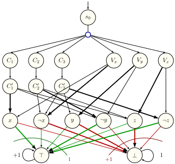
Proof sketch. We provide a reduction from 3-SAT [Karp, 1972]; full details of the construction and correctness proof appear in the full version [Bahmani et al., 2026]. Given a 3-SAT instance ϕ over variables X = {x1, . . . , xn} and clauses C = {C1, . . . , Cm}, we construct an asymmetricallydiscounted MDPMϕ with two principals such that the optimal social welfare is non-negative iff ϕ is satisfiable. See Figure 2 for an illustrative example. Let L = X ∪{¬x : x ∈ X} be the set of literals.

Construction. The MDP has an initial state s0 with a single action that leads, with probability 1 n+m , to each state in C ∪ {Vx : x ∈ X}; this is the only probabilistic transition. From each clause state Ci, a single action leads to its duplicate C ′ i in C ′ = {C ′1 , . . . ,C ′m}. From each C ′ i , there is one action for each literal ℓ in clause Ci, leading to the state ℓ ∈ L.

Algorithm 1 Compute long-term strategy for optimal welfare

• 1: Input : M
• 2: Output: MDP with long-term strategies and evaluation
• 3: M0 ←M
• 4: for j ∈ {0, · · · , n-1} do
• 5: Vj ←optimal values for Principal j inMj
• 6: Mj+1 ←Mj restricted to actions with a strategy optimal for Principal j inMj
• 7: end for
• 8: Output: Restricted MDP Mn and value functions V0, . . . , Vn-1

Similarly, from each variable state Vx, there are two actions, leading respectively to x and ¬x. From each literal state ℓ ∈ L, two actions choose between the sink states ⊤ and ⊥, each of which has a single self-loop action.

Rewards and discounting. The two principals have discount factors 0.54 and 0.4, respectively, and identical rewards. At each literal state ℓ ∈ L, choosing ⊤ gives reward -1, while choosing ⊥ gives reward +1. At the sink states, staying in ⊤ gives reward +1, and staying in ⊥ gives reward -1. All other actions have reward 0.

Correctness intuition. The construction ensures that satisfying assignments correspond to strategies that direct short paths to low-reward sinks and long paths to high-reward sinks, aligning reward trajectories with the structure of ϕ. The chosen discount factors ensure that only such satisfying strategies yield social welfare above the threshold.

4 ComputingWelfare-Optimal Strategies

In this section, we present a polynomial-time algorithm for synthesising a joint strategy that maximises social welfare in a given asymmetrically-discounted MDP.

We begin by outlining our algorithm and the underlying intuition. The key insight is that there always exists a positional strategy that can be adopted after a finite number of steps without loss of optimality. Our algorithm first identifies such a limit strategy. Next, we show that the number of steps required before switching to this limit strategy is polynomial in the size of the MDP. By unrolling the MDP into a directed acyclic graph (DAG) up to this horizon and evaluating it backward, we obtain a simple and efficient construction of welfare-optimal strategies. These strategies are pure, finite-memory, and rely only on a counter. We conclude the section by establishing that computing the optimal social welfare in asymmetrically-discounted MDPs is P-complete.

4.1 Asymptotic Strategy Behaviour

We begin by computing a long-term strategy by solving the MDP from the perspective of Principal 0-the most patient principal (highest discount factor). Since this reduces to a standard single-agent MDP with a discounted reward objective, optimal state values and corresponding actions can be computed in polynomial time [Puterman, 1994]. In general, multiple actions may yield the same optimal value in a given state. To resolve such ties, we sequentially invoke the preferences of the remaining principals as tie-breakers: first Principal 1, then Principal 2, and so on, following the order of increasing patience. This is formalised in Algorithm 1.

Let Vi : S → Q denote the value function for Principal i in the MDPMi, where Mi is the MDP restricted to the remaining admissible actions after resolving ties at the previous levels. The reason for correctness is that, due to faster discounting, an advantage of a principal with a lower discount factor will eventually be dwarfed by a disadvantage of a principal with a higher discount factor. We do not have to prove this at this point; instead, we will later show that deviation from this strategy will eventually be unattractive.

Lemma 1. Algorithm 1 runs in time polynomial in its input.

It follows because the procedure evaluates n MDPs, each of which can be evaluated in polynomial time [Puterman, 1994].

4.2 Deviations fromAsymptotic Behaviour

As illustrated by example 1 in the introduction-where the long-term strategy prescribes always selecting action b-it can be advantageous for social welfare to initially deviate from the asymptotic strategy. Specifically, a deviation in the very first step (i.e., after zero steps) may yield improved outcomes for certain principals. To quantify the impact of such a deviation, we define the payoff difference for Principal i resulting from taking action a in state s, instead of following the long-term strategy. This difference [Baird and Leemon, 1993; Sutton and Barto, 2018] is given by:

where Vi(s) denotes the value of state s under the optimal strategy for Principal i in the corresponding one-principal MDPMi. If the same happens after j-steps, the payoff difference is

Note that we now have

We now only need to argue that, for reasonably spaced discount factors, there is a small κ s.t., for all j > κ, ∑n-1 i=0 ∆j(sj, aj, i) ≤ 0 holds. Once this is the case, we can optimise social welfare by never deviating from Mn from this point onwards.

Observation 1. For all states s ∈ S and all actions a ∈ A(s) for Mn, all i ∈ P , and j ∈ N0, we have ∆j(s, a, i) = 0. For all actions a ∈ A(s) for M, but not for Mn, we have that there is a minimal i such that ∆0(s, a, i) ̸= 0; and for this i, ∆0(s, a, i) < 0 holds.

Lemma 2. For all s ∈ S, a ∈ A(s), i ∈ P, j ∈ N0, we have

Proof. This can be shown by a simple inductive argument with trivial basis (k = j) and induction step k ↦→ k + 1 as

for ℓ ≤ i, where the sums are non-positive by the induction hypothesis.

As the Vi returned by Algorithm 1 are the solution to a system of linear equations defined by any remaining strategy in Mn, their values are fractions with both the numerator and the denominator singly exponential (in value, and polynomial in length) in the input to the algorithm. Thus, to estimate κ, when we take such a ∆0(s, a, i) < 0, then κ′s,a = ∑n-1 j=i+1 max{0,∆0(s, a, j)}/|∆0(s, a, i)| , is exponentially bounded by value, and polynomially by length, in the input to Algorithm 1. It is now easy to see that 1 , for

and j ≥ κs,a, ∑n-1 i=0 ∆j(s, a, i) ≤ 0 holds. For an action a ∈ A(s) for Mn, we have ∆j (s, a, i) = 0 for all principals i and all j ∈ N0, so we choose κs,a = 0. We set κ = max{κs,a | s ∈ S, a ∈ A(s)} to the maximal value among the κs,a, so that, for all j ≥ κ, ∑n-1 i=0 ∆j(s, a, i) ≤ 0 holds.

Lemma 3. No higher social welfare can be obtained by deviating from the strategies available inMn after κ steps (as defined above). If the discount factors are reasonably spaced, κ is polynomial in the size of the input to Algorithm 1.

Proof. For the first part of the claim, we note that κ is chosen so that the initial sums from Lemma 2 are all non-positive. Thus, for j ≥ κ steps, all expected sums E ∑n-1 i=0 ∆j(sj, aj, i) from Equation 6 are non-positive and are zero if, and only if, the chance of taking an action available in Mn is one. For the second part, it is clear that each lnκ′s,a is polynomially bounded, while Assumption 1 provides that the reciprocal of the denominator ln(λi/λi+1) is also polynomially bounded.

4.3 Computing Social Welfare

In order to find the social welfare (and a strategy that achieves it), we consider Algorithm 1 again and note that we have already determined ∑n-1 i=0 Vi(s) and showed that we have to followMn after κ steps as defined in the previous sectionwhere we also showed that ∑∞j=κ E ∑n-1 i=0 ∆j(sj, aj, i) = 0 for social welfare. To maximise social welfare, maximise:

To do this, we can simply unravel the MDP M = (S, A, T, P, R, Λ) to a finite DAG

1 This skips over the corner case of i = n - 1; in that case, ∑n-1 i=0 ∆j(s, a, i) < 0 holds for all j ∈ N0 and we set κs,a = 0.

on the fly, where, for j < κ - 1, A′ (s, j) = A(s), T ′ (s, j, a)(s′ , j + 1) = T(s, a)(s′ ), and R′ (s, j, a) = ∑i∈P ∆j(s, a, i), while A′ (s, κ - 1) = ∅. Note that we do not calculate κ, but stop unravelling once, for all s ∈ S and all a ∈ A(s) all initial sums of ∑i′ i=0 ∆j (s, a, i) are nonpositive, which Lemma 2 shows to henceforth holds forever, while Lemma 3 shows that this happens after a few iterations.

Lemma 4. An optimal total reward strategy σ for the DAG MDP D (followed by any stay-in-Mn strategy) defines a finite counting strategy σ′ for M that provides optimal social welfare. Moreover, if its expected reward for the initial strategy on D for a state (s, 0) is Eσ(s, 0), then the social welfare for a starting state s is SWσ′ = ∑n-1 i=0 Vi(s) +Eσ(s, 0).

Proof. By construction of D, its optimal solutions maximise ∑κ-1 j=0 E ∑n-1 i=0 ∆j(sj, aj, i), and κ is selected so that, by Lemma 2, ∑n-1 i=0 ∆j(s, a, i) ≤ 0 for all j ≥ κ, while following Mn provides ∑n-1 i=0 ∆j(s, a, i) = 0. The value for SWσ′ can be obtained from Equation 6.

4.4 Complexity

The preceding results yield the following complexity classification. For reasonably spaced discount factors, welfare optimisation is polynomial-time solvable, while the associated decision problem remains P-complete. Here, SOCIALWELFARE asks whether there exists a strategy σ whose social welfare is non-negative.

Theorem 2. The social welfare of an asymmetricallydiscounted MDPMwith reasonably spaced discount factors can be computed in polynomial time. Moreover, SOCIALWELFARE is P-complete, even when restricted to two-player zero-sum games or single-player MDPs.

Proof. For inclusion in P, we have shown that our algorithm terminates with the social welfare (cf. Lemma 4). To obtain this, we first run Algorithm 1 to obtain the long-term values and strategy time polynomial in the input to Algorithm 1 (cf. Lemma 1). We then unravel M, replacing the reward after j steps by R(s, a, j) = ∑n-1 i=0 ∆j(s, a, i). Each unravelling step is cheap, and for reasonably spaced discount factors, we are guaranteed to stop unravelling after a polynomial number of steps (cf. Lemma 3) into an MDP D with a DAG structure.

Analysing D can then be done layer by layer: for states in the final layer κ, the expected payoff is E(s, κ) = 0 (as the end of the DAG has been reached). Once a layer j+1 is evaluated, we can locally evaluate

This can be done in time polynomial in D (and inM) when discount factors are reasonably spaced (cf. Lemma 3).

For hardness, we reduce from reachability games [Immerman, 1999] on alternating graphs. In an alternating graph, the reachability player controls the OR nodes, while the safety player controls the AND nodes. We translate the game nodes to states, translating OR nodes to states with one action, so that T picks among the successors of that node uniformly at

• (a) Up to 2K states.

(b) 3 to 105 states, without Algo.1.

• (c) Varying principals.
• (d) Varying discount spacing.

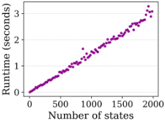
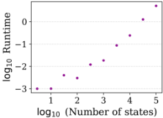
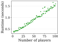
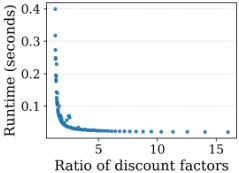
Figure 3: Running time grows linearly with the states in reasonably sized MDPs with up to 2K states; remains linear, without Algorithm 1, across MDPs with 3 to 105 states; grows linearly with the number of principals; and falls as the factor between discount factors grows.

random. We translate AND nodes to states with as many actions as it has successors and let the MDP freely pick to which successor state it moves. For payoffs, we use R(t, a) = -1 for all a ∈ A(t), and R(s′ , a) = 0 otherwise.

If the safety player can win, she can win with a positional strategy in the reachability game; the same strategy provides a social welfare of 0, which is optimal as no individual payoff is positive. Vice versa, a strategy σ that provides SWσ = 0 in the resulting MDP provides a winning strategy for the safety player in the reachability game. Finally, if we consider two-player zero-sum games instead, we use the payoffs R(t, a, 0) = -1, R(t, a, 1) = +1, and R(t, a, i) = 0 otherwise and retain the same argument.

5 Experimental Results

We study scalability through three research questions (RQs): (RQ1) the number of states, (RQ2) the number of principals, and (RQ3) the spacing of discount factors. For each question, we construct randomised MDP families with structural features designed to expose the relevant performance trends. The results demonstrate the empirical tractability of our method across these key dimensions of complexity.

Experiments ran on a Linux workstation with an Intel i74790 CPU at 3.60GHz, 8 cores, and 8.2GB RAM, using Python 3.12.3 and glibc 2.39. Additional plots and runtime comparisons, including runs with and without MDP-solving, appear in the full version [Bahmani et al., 2026].

RQ1: Scalability with size of MDPs. To evaluate scalability with respect to the number of states, we designed two sets of experiments: first, we generated 100 randomised MDP instances, varying the number of states from 2 to 2000 in increments of 20. Each MDP has two principals with fixed discount factors (0.9, 0.3), and two actions per state. Figure 3 (left) shows that as the number of states in the MDPs increases (from 2 to 2000), the time required to calculate the optimal social welfare grows linearly with the size of the MDP, demonstrating scalability in relation to the number of states. Second, to assess scalability on large-scale MDPs, we evaluated the algorithm on a smaller set of instances with larger state spaces. We generated MDPs with the number of states ranging from 3 to 105 , using powers of √10. Each MDP consisted of 6 principals with fixed discount factors and 2 actions per state. Figure 3 (mid-left) shows that the algorithm remains tractable even for large MDPs. In this plot only, we exclude the runtime of Algorithm 1, because MDP solving dominates the cost and becomes the bottleneck.

RQ2: Scalability with the number of principals. To evaluate scalability with respect to the number of principals, we generated 100 randomised MDP instances, varying the number of principals from 2 to 101 in increments of 1 principal per example. Each MDP had a fixed number of 30 states, and exactly two actions per state. The principals' discount factors formed an arithmetic progression from 0.99 (most patient) to 0.05 (least patient) according to λi = 0.99-(i-1) 0.94 n-1 . Figure 3 (mid-right) shows that the computational time required to compute optimal social welfare grows polynomially with the number of principals, demonstrating scalability of the algorithm in relation to the number of principals.

RQ3: Scalability with the ratio of discount factors. To evaluate scalability with respect to the ratio of discount factors of principals ( λ0 /λ1), we generated 100 randomised MDP instances, varying the ratio of discount factors from 1.32 (almost identical patience) up to 16 (strongly asymmetric patience). Each MDP had two principals, fixed number of 30 states, and exactly two actions per state. Figure 3 (right) shows that the execution time falls steeply as the ratio grows: runs start at ≈ 0.3s when the two discount factors are nearly equal ( λ0 λ1 = 1.32), drop below 0.02s when λ0 λ1 ≈ 4, and then flatten out around 0.01s for when λ0 λ1 = 16.

6 Conclusion

We introduced asymmetrically-discounted MDPs as a natural model for decision-making on behalf of multiple principals with heterogeneous time preferences. We showed that socialwelfare-optimal strategies can be computed tractably under reasonable assumptions on discount-factor spacing, and that such optima can be realised by pure, finite-memory strategies.

Our results highlight the computational and strategic complexity introduced by temporal asymmetries, and open new directions for multi-agent planning, algorithmic game theory, and the study of intertemporal incentives.

Acknowledgements

This work was supported by the EPSRC through grants EP/X03688X/1 (TRUSTED) and EP/X042596/1 (Games for Good), and in part by the NSF under CAREER Award CCF2146563. Ashutosh Trivedi is a Royal Society Wolfson Visiting Fellow and gratefully acknowledges the support of the Wolfson Foundation and the Royal Society.