
Frequency-Aware Augmentation and Alignment for Time Series Contrastive Learning
Proceedings of the Thirty-Fifth International Joint Conference on Artificial Intelligence. Main Track. Pages 2879-2887.
https://doi.org/10.24963/ijcai.2026/320
Keywords
- Data Mining: Mining spatial and/or temporal data
- Machine Learning: Self-supervised Learning
- Machine Learning: Unsupervised learning
Abstract
Contrastive learning has become a dominant paradigm for learning time series representations from large-scale unlabeled data. However, current methods are often adapted from computer vision and rely on random time-domain augmentations (e.g., jittering and cropping). Such augmentations can unpredictably disrupt the natural frequency structure of signals, leading to representations failing to capture crucial patterns in the data. To address this, we propose a framework of Frequency-Aware Augmentation and Alignment for Time Series Contrastive Learning (FACL), which comprises two key innovations. First, FACL employs a novel frequency-structured augmentation mechanism based on wavelet transforms. The mechanism constructs controlled and interpretable contrastive views by the structured attenuation and recombination of specific wavelet components. Second, FACL introduces a multi-level contrastive objective that incorporates a subspace alignment strategy. This objective explicitly aligns representations within their corresponding frequency subspaces. Experiments across six forecasting and four classification benchmarks show that FACL achieves superior performance compared to recent baselines. Ablation studies and model analysis highlight the contribution of each component in FACL. Furthermore, low-sample semi-supervised learning experiments confirm the robustness and generalization of FACL.
- [Alimoglu and Alpaydin, 2001] Fevzi Alimoglu and Ethem Alpaydin. Combining multiple representations for pen- based handwritten digit recognition. Turkish Journal of Electrical Engineering and Computer Sciences, 9(1):1- 12, 2001.
- [Andrzejak et al., 2001] Ralph G Andrzejak, Klaus Lehn- ertz, Florian Mormann, Christoph Rieke, Peter David, and Christian E Elger. Indications of nonlinear deterministic and finite-dimensional structures in time series of brain electrical activity: Dependence on recording region and brain state. Physical Review E, 64(6):061907, 2001.
- [Anguita et al., 2013] Davide Anguita, Alessandro Ghio, Luca Oneto, Xavier Parra, Jorge Luis Reyes-Ortiz, et al. A public domain dataset for human activity recognition using smartphones. In Esann, volume 3, pages 3-4, 2013.
- [Blankertz et al., 2001] Benjamin Blankertz, Gabriel Curio, and Klaus-Robert Müller. Classifying single trial eeg: To- wards brain computer interfacing. Advances in neural in- formation processing systems, 14, 2001.
- [Chang et al., 2024] Ching Chang, Chiao-Tung Chan, Wei- Yao Wang, Wen-Chih Peng, and Tien-Fu Chen. Time- drl: Disentangled representation learning for multivariate time-series. In 2024 IEEE 40th International Conference on Data Engineering (ICDE), pages 625-638. IEEE, 2024.
- [Chen et al., 2020] Ting Chen, Simon Kornblith, Moham- mad Norouzi, and Geoffrey Hinton. A simple framework for contrastive learning of visual representations. In In- ternational conference on machine learning, pages 1597- 1607. PMLR, 2020.
- [Chen et al., 2023] Xi Chen, Cheng Ge, Ming Wang, and Jin Wang. Supervised contrastive few-shot learning for high- frequency time series. In Proceedings of the AAAI Con- ference on Artificial Intelligence, volume 37, pages 7069- 7077, 2023.
- [Cheng et al., 2026] Mingyue Cheng, Xiaoyu Tao, Zhiding Liu, Qi Liu, Hao Zhang, Rujiao Zhang, and Enhong Chen. Timemae: Self-supervised representations of time series with decoupled masked autoencoders. In Proceedings of the Nineteenth ACM International Conference on Web Search and Data Mining, pages 498-508, 2026.
- [Dong et al., 2023] Jiaxiang Dong, Haixu Wu, Haoran Zhang, Li Zhang, Jianmin Wang, and Mingsheng Long. Simmtm: A simple pre-training framework for masked time-series modeling. Advances in Neural Information Processing Systems, 36, 2023.
- [Duan et al., 2024] Jufang Duan, Wei Zheng, Yangzhou Du, Wenfa Wu, Haipeng Jiang, and Hongsheng Qi. Mf- clr: multi-frequency contrastive learning representation for time series. In Proceedings of the 41st International Conference on Machine Learning, pages 11918-11939, 2024.
- [Eldele et al., 2021] Emadeldeen Eldele, Mohamed Ragab, Zhenghua Chen, Min Wu, Chee Keong Kwoh, Xiaoli Li, and Cuntai Guan. Time-series representation learning via temporal and contextual contrasting. International Joint Conference on Artificial Intelligence, 2021. IJCAI
- [Franceschi et al., 2019] Jean-Yves Franceschi, Aymeric Dieuleveut, and Martin Jaggi. Unsupervised scalable rep- resentation learning for multivariate time series. Advances in neural information processing systems, 32, 2019.
- [Fu and Hu, 2025] En Fu and Yanyan Hu. Frequency- masked embedding inference: A non-contrastive approach for time series representation learning. In Proceedings of the AAAI Conference on Artificial Intelligence, volume 39, pages 16639-16647, 2025.
- [Lai et al., 2018] Guokun Lai, Wei-Cheng Chang, Yiming Yang, and Hanxiao Liu. Modeling long-and short-term temporal patterns with deep neural networks. In The 41st international ACM SIGIR conference on research & devel- opment in information retrieval, pages 95-104, 2018.
- [Liu et al., 2024] Zihan Liu, Bowen Du, Junchen Ye, Xian- qing Wen, and Leilei Sun. An ncde-based framework for universal representation learning of time series. In Pro- ceedings of the Thirty-Third International Joint Confer- ence on Artificial Intelligence, pages 4623-4633, 2024. IJCAI
- [Liu et al., 2026] Yusen Liu, Zhichen Lai, Hua Lu, Xu Cheng, Tianqing Zhu, Xiufeng Liu, and Huan Huo. Saurl-ts: A self-adaptive framework for unsu- pervised time series representation learning. Pattern Recognition, page 113129, 2026.
- [Luo et al., 2023] Dongsheng Luo, Wei Cheng, Yingheng Wang, Dongkuan Xu, Jingchao Ni, Wenchao Yu, Xuchao Zhang, Yanchi Liu, Yuncong Chen, Haifeng Chen, and Xiang Zhang. Time series contrastive learning with information-aware augmentations. In Proceedings of the AAAI Conference on Artificial Intelligence, volume 37, pages 4534-4542, 2023.
- [Meng et al., 2023] Qianwen Meng, Hangwei Qian, Yong Liu, Lizhen Cui, Yonghui Xu, and Zhiqi Shen. Mhccl: masked hierarchical cluster-wise contrastive learning for multivariate time series. In Proceedings of the AAAI Con- ference on Artificial Intelligence, volume 37, pages 9153- 9161, 2023.
- [Nie et al., 2022] Yuqi Nie, Nam H Nguyen, Phanwadee Sinthong, and Jayant Kalagnanam. A time series is worth 64 words: Long-term forecasting with transformers. arXiv preprint arXiv:2211.14730, 2022.
- [Oord et al., 2018] Aaron van den Oord, Yazhe Li, and Oriol Vinyals. Representation learning with contrastive predic- tive coding. arXiv preprint arXiv:1807.03748, 2018.
- [Sharma et al., 2020] Vivek Sharma, Makarand Tapaswi, M Saquib Sarfraz, and Rainer Stiefelhagen. Clustering based contrastive learning for improving face representa- tions. In 2020 15th IEEE International Conference on Au- tomatic Face and Gesture Recognition (FG 2020), pages 109-116. IEEE, 2020.
- [Tonekaboni et al., 2021] Sana Tonekaboni, Danny Eytan, and Anna Goldenberg. Unsupervised representation learn- ing for time series with temporal neighborhood coding. International Conference on Learning Representations, 2021.
- [Woo et al., 2022] Gerald Woo, Chenghao Liu, Doyen Sa- hoo, Akshat Kumar, and Steven Hoi. Cost: Contrastive learning of disentangled seasonal-trend representations for time series forecasting. International Conference on Learning Representations, 2022.
- [Wu et al., 2024] Yuhan Wu, Xiyu Meng, Yang He, Junru Zhang, Haowen Zhang, Yabo Dong, and Dongming Lu. Multi-view self-supervised contrastive learning for multi- variate time series. In Proceedings of the 32nd ACM In- ternational Conference on Multimedia, pages 9582-9590, 2024.
- [Yang et al., 2024] Runze Yang, Longbing Cao, Jianxun Li, and Jie Yang. Rethinking fourier transform from a basis functions perspective for long-term time series forecast- ing. Advances in Neural Information Processing Systems, 37:8515-8540, 2024.
- [Yue et al., 2022] Zhihan Yue, Yujing Wang, Juanyong Duan, Tianmeng Yang, Congrui Huang, Yunhai Tong, and Bixiong Xu. Ts2vec: Towards universal representation of time series. In Proceedings of the AAAI Conference on Ar- tificial Intelligence, volume 36, pages 8980-8987, 2022.
- [Zhang et al., 2022] Xiang Zhang, Ziyuan Zhao, Theodoros Tsiligkaridis, and Marinka Zitnik. Self-supervised con- trastive pre-training for time series via time-frequency consistency. Advances in Neural Information Processing Systems, 35:3988-4003, 2022.
- [Zhang et al., 2024] Kexin Zhang, Qingsong Wen, Chaoli Zhang, Rongyao Cai, Ming Jin, Yong Liu, James Y Zhang, Yuxuan Liang, Guansong Pang, Dongjin Song, et al. Self-supervised learning for time series analysis: Taxonomy, progress, and prospects. IEEE transactions on pattern analysis and machine intelligence, 46(10):6775- 6794, 2024.
- [Zheng et al., 2023] Xiaochen Zheng, Xingyu Chen, Manuel Schürch, Amina Mollaysa, Ahmed Allam, and Michael Krauthammer. Simts: Rethinking contrastive representa- tion learning for time series forecasting. arXiv preprint arXiv:2303.18205, 2023.
- [Zheng et al., 2024] Xu Zheng, Tianchun Wang, Wei Cheng, Aitian Ma, Haifeng Chen, Mo Sha, and Dongsheng Luo. Parametric augmentation for time series contrastive learn- ing. International Conference on Learning Representa- tions, 2024.
- [Zhou et al., 2021] Haoyi Zhou, Shanghang Zhang, Jieqi Peng, Shuai Zhang, Jianxin Li, Hui Xiong, and Wan- cai Zhang. Informer: Beyond efficient transformer for long sequence time-series forecasting. In Proceedings of the AAAI conference on artificial intelligence, volume 35, pages 11106-11115, 2021.
- [Zhou et al., 2022] Tian Zhou, Ziqing Ma, Qingsong Wen, Xue Wang, Liang Sun, and Rong Jin. Fedformer: Fre- quency enhanced decomposed transformer for long-term series forecasting. In International conference on machine learning, pages 27268-27286. PMLR, 2022.
- [Zhou et al., 2024] Shuang Zhou, Daochen Zha, Xiao Shen, Xiao Huang, Rui Zhang, and Korris Chung. Denoising- aware contrastive learning for noisy time series. In Pro- ceedings of the Thirty-Third International Joint Confer- ence on Artificial Intelligence, pages 5644-5652, 2024.
References were extracted automatically from the PDF and may contain errors.
Full text extracted automatically from the PDF; figures, tables and equations may differ. The PDF is the version of record.
1 Introduction
Time series data arises in various domains, capturing the dynamics of complex systems in finance, healthcare, climate science, and industrial IoT. However, obtaining largescale labeled datasets is expensive and often infeasible. Selfsupervised learning has become a promising alternative by leveraging large amounts of unlabeled data to learn robust and transferable representations for downstream tasks [Zhang et al., 2024]. Among self-supervised methods, contrastive learning has become popular. It essentially learns representations from multiple augmented views of each sequence by enforcing alignment in the latent space.
∗Corresponding authors.
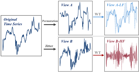
However, most time series contrastive learning methods [Tonekaboni et al., 2021; Yue et al., 2022] rely on random time-domain augmentations (e.g., jittering, cropping, and scaling) that are adapted from computer vision [Oord et al., 2018; Chen et al., 2020]. While these augmentations work well for visual data, they may distort the underlying patterns in time series. In particular, random augmentations can unpredictably disrupt the natural frequency structure of signals. Moreover, most methods focus only on global features, which are typically dominated by low-frequency patterns, and ignore frequency-specific details. As a result, the learned representations often lack awareness of meaningful frequency components. Although recent work has explored automatic augmentation [Luo et al., 2023; Zheng et al., 2024] and the use of frequency-domain signals [Zhang et al., 2022; Woo et al., 2022; Wu et al., 2024], two challenges remain:
First, random augmentations distort key frequency components of time series signals. Time series signals exhibit patterns across multiple frequency components, including slow-moving trends at low frequency, seasonal cycles at mid frequency, and fine-grained details and noise at high frequency. Time-domain random perturbations can unpredictably disrupt or remove one or more of these components; some augmentations cause severe distortion of low-frequency information, while others significantly reduce the energy in the mid- and high-frequency bands. As shown in Figure 1, the original time series from the ETTm1 dataset is subjected to two types of random augmentations to generate two augmented views. A stronger augmentation, Permutation, produces View A, while a milder augmentation, Jitter, produces View B. A wavelet transform (WT) is applied to each view to decompose it into multiple frequency components. From View A, the low-frequency component is reconstructed back to the time domain (View A-LF). The original low-frequency trend, shown as the solid line, is disrupted and replaced by a modified version indicated by the lighter dashed line. Similarly, the high-frequency component (View B-HF) is reconstructed from View B, and the original fine-grained details are distorted, resulting in altered high-frequency content.
Second, the standard contrastive pretext task is blind to frequency sub-structures. Contrastive learning, as a typical self-supervised pretext task, learns representations by aligning information across different augmented views of the same input. However, when contrastive learning enforces similarity only on global representations, the alignment is largely driven by dominant low-frequency components, such as overall trends. As a result, the model can reduce the contrastive loss largely by matching the overall trend between views, while neglecting the alignment of finer-grained, high-frequency components. This leads to suboptimal representations for downstream tasks that require sensitivity to these components. In time series forecasting, explicitly modeling selected mid- and high-frequency components can improve the stability and accuracy of long-range predictions [Zhou et al., 2022; Yang et al., 2024]. For example, the ETTm1 and ETTm2 subsets record transformer oil temperature and load at 15-minute intervals over a two-year period. To achieve accurate predictions on such data, models must capture high-frequency variations and short-term spikes, which are easily missed under standard contrastive objectives.
To address these issues, we propose FACL, a contrastive learning framework that incorporates frequency-aware augmentation and alignment for time series. FACL first introduces a frequency-structured view construction mechanism based on wavelet decomposition. This approach decomposes the original signal into multiple interpretable and reconstructible frequency sub-bands. By structurally attenuating and recombining these frequency bands, the generated contrastive views preserve all band-specific information in a controlled manner and avoid the distortions caused by random augmentations. Moreover, FACL proposes a frequency subspace alignment strategy. The constructed views are first processed by a customized encoder to extract multi-scale frequency features, which are then projected into their corresponding frequency subspaces. Beyond the global-level contrastive loss, FACL introduces an intra-contrastive loss that aligns diverse frequency information within each subspace. This multi-level contrastive objective complements the global loss by explicitly encouraging consistency across frequency-specific representations, enabling better modeling of frequency-dependent patterns.
In summary, our main contributions are as follows:
- We propose a frequency-structured view construction mechanism that preserves frequency-domain structures in a controlled manner and provides interpretable contrastive views.
- We propose a frequency subspace alignment strategy that drives the model to capture crucial frequencyspecific features beyond global-level alignment.
- Extensive experiments demonstrate that our framework outperforms state-of-the-art contrastive learning methods on both forecasting and classification benchmarks, and further validate the effectiveness of each component.
2 ProblemFormulation
Let X = {xi}Ni=1 be a dataset of N unlabeled time series samples. Each sample is a time series x ∈ RT×C , where T is the sequence length and C is the number of variables. Our objective is to learn an encoder fθ : RT×C → RT×d that maps an input time series x to a d-dimensional representation h = fθ(x), which captures the temporal and structural patterns of x. In the self-supervised contrastive learning setting, fθ is trained using a contrastive pretext task that leverages the intrinsic structure of the data. Specifically, for each input x, a pair of views (˜x1, ˜x2) is generated via data augmentations, denoted as ˜x1 = A1(x) and ˜x2 = A2(x), where A1 and A2 are sampled from a family of augmentation operators A. We treat (˜x1, ˜x2) as a positive pair and contrast them with other views in the batch, which serve as negatives. This process trains fθ to align semantically meaningful information across different augmented views, enabling it to learn representations that are useful for downstream tasks.
3 Methodology
In this section, we first present an overview of the FACL framework and then detail its two main components: a frequency-structured view construction mechanism and a frequency subspace alignment strategy.
3.1 Overview
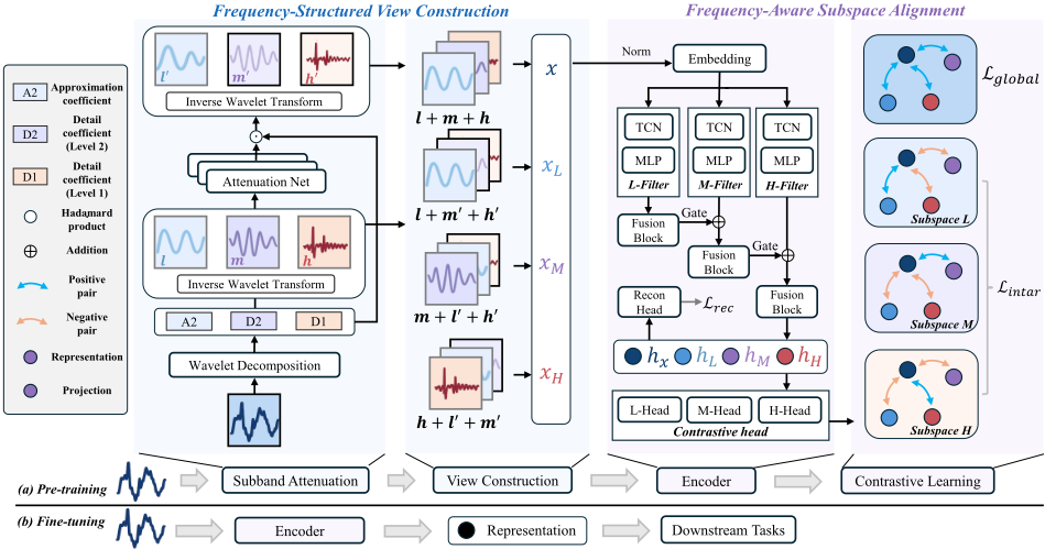
Figure 2 provides an overview of the proposed FACL framework. The pre-training pipeline begins with subband attenuation and view construction, where each input time series is decomposed into subbands using the discrete wavelet transform (DWT). A learnable attenuation network is applied to selected subbands, followed by an inverse transform to reconstruct and recombine them into multiple augmented views. The generated views are subsequently processed by a frequency-aware encoder, which extracts feature representations from them. The encoder employs parallel dilated convolutional branches, followed by a gated fusion module that integrates the features into a unified embedding. Finally, FACL is trained with a multi-level objective composed of three parts: (i) a global contrastive loss that aligns overall sequence representations across views, (ii) an intracontrastive loss that aligns subbands within their corresponding frequency subspaces, and (iii) a reconstruction loss that constrains distortion and preserves key information.
3.2 Frequency-Structured ViewConstruction
Random augmentations from computer vision, such as jitter, scaling, and permutation, often distort time series frequency content in uncontrolled ways. To address this, we propose a frequency-structured view construction mechanism that generates views with explicit frequency semantics.
Wavelet Decomposition. Given an input time series x ∈ RT×C , we apply a DWT with two decomposition levels. Let W denote the forward DWT operator and W-1 its inverse. A two-level DWT produces three sets of coefficients, namely A2 (the approximation coefficients), D2 (the detail coefficients at level 2), and D1 (the detail coefficients at level 1).
These coefficients correspond to different scales in the multiresolution decomposition, each emphasizing signal content within a specific frequency range. Specifically, A2 captures coarse-scale structures associated with low-frequency trends, D2 reflects variations at an intermediate scale, and D1 highlights fine-scale details typically linked to higherfrequency components. Under the theoretical guarantee of wavelet transform invertibility, the original signal can be exactly reconstructed from its decomposition coefficients using the inverse transformW-1 :
Attenuation Networks. To enable frequency-specific perturbations, we introduce a set of learnable attenuation networks, each dedicated to one wavelet subband. Collectively denoted as rϕ, these networks share the same structure, which consists of a multi-layer perceptron followed by a sigmoid activation. The collection rϕ takes the wavelet coefficients from all subbands as input:
Each output αA2 , αD2 , αD1 is an element-wise scaling mask with the same shape as its corresponding wavelet coefficient subband, with values constrained to the range (0, 1). These masks control the degree of attenuation applied to the approximation and detail coefficients. We then apply each mask to its corresponding wavelet coefficients to obtain the attenuated subband components:
Here, ˜ A2, ˜D2, ˜D1 denote the wavelet coefficients after applying frequency-specific attenuation.
View Construction. Based on the original wavelet coefficients (A2,D2,D1) and their attenuated counterparts ( ˜ A2, ˜D2, ˜D1), we construct one anchor view and three perturbed views. Each view is constructed following a two-band attenuation principle, in which exactly one frequency band is preserved while the other two are attenuated.
This design is grounded in the invertibility of the wavelet transform: for a two-level decomposition, all three components (A2,D2,D1) are required to reconstruct the original signal, and having these three components alone is sufficient for an exact reconstruction, as shown in Eq. (2). For clarity, as shown in Figure 2, we present our view construction process in the time domain. We apply the inverse wavelet transform to each component (A2,D2,D1) separately, obtaining three time-domain signals (l,m, h), respectively. Similarly, their attenuated counterparts are denoted as (l′ , m′ , h′ ).
Assuming a linear, perfect-reconstruction wavelet transform, the original signal can be losslessly recovered by summing the components: x = l + m + h. Leveraging this property, we construct three augmented views by recombining the attenuated and unattenuated components: (i) xL = l +m′ + h′ , which preserves the low-frequency component, (ii) xM = l′ +m+ h′ , which preserves the mid-frequency component, and (iii) xH = l′ +m′ + h, which preserves the high-frequency component. By selectively attenuating two components while retaining one, each view emphasizes a distinct frequency range, and the preserved content of each view is explicitly controlled and interpretable. Equivalently, we use a more convenient implementation to generate the views:
Based on Eqs. (2), (5)-(7), we obtain the anchor sequence x as well as three frequency-structured views xL, xM, and xH. Each view isolates a distinct portion of the frequency spectrum, which enhances interpretability and provides wellstructured signals for contrastive learning.
3.3 Frequency-Aware Subspace Alignment
Once the views are constructed, the next step is to extract representations and align them across the corresponding frequency subspaces. To this end, we introduce a unified encoder and a multi-level contrastive objective.
Feature Extraction. As shown in Figure 2, the encoder fθ is designed to capture multi-scale features. We adopt a temporal convolutional network (TCN) architecture with parallel band-specific processing streams and gated fusion.
For each input (anchor or augmented view), the encoder applies per-channel normalization and embeds it into a latent space. To capture multi-frequency patterns, it uses three parallel TCN branches with distinct dilation rates, each followed by an MLP. This multi-branch design enables the encoder to extract multi-scale features. These features are then integrated progressively through a gated mechanism. The fusion begins with uL (L-Filter output), which is passed through the first fusion block (an MLP). The resulting representation is combined with uM (M-Filter output) using a learned gating weight γ L, predicted by an MLP, and then processed by the second fusion block. Finally, this feature is fused with uH (H-Filter output) via another gating weight γM and passed through the third fusion block, yielding the final fused representation h. This progressive fusion strategy produces frequency-aware representations that support the subsequent alignment objective. For simplicity, we denote this as:
where hx denotes the anchor representation, and hL, hM, and hH correspond to the three views.
Global Loss. For the global contrastive loss, all views from the same anchor form positive pairs, and the loss function serves to pull their representations closer in the global latent space. Formally, given a batch B ⊆ X, for each sample x ∈
B, the loss is defined using InfoNCE [Oord et al., 2018]:
where sim(·, ·) denotes cosine similarity, τ is the temperature for the global loss, V(x) is the view set of anchor x (i.e., {xL, xM, xH}), and Ng is the global negative set, consisting of all augmented views from other samples in the batch B. Iterating over all samples as anchors enforces bidirectional alignment between each sequence and its views.
Frequency Subspace Alignment. To align representations across frequency subspaces, the anchor and views are projected into latent spaces via distinct MLP projection heads. Because of the frequency-structured view construction, each view shares exactly one frequency band with the anchor, which enables targeted alignment within that subspace.
In each frequency subspace s ∈ S = {L,M,H}, let zsx denote the projection of the anchor sequence x. Similarly, let zsk denote the projection of a constructed view xk (where k ∈ {L,M,H}) into the same subspace s. Here, the superscript s indicates the target subspace, while the subscript k identifies the frequency band preserved by the view. Targeted alignment is achieved by matching the anchor with the view that retains the corresponding frequency information. Therefore, within subspace s, the projection where k = s forms the positive pair with the anchor (denoted as zs s ), while projections from the other views (k ̸= s) serve as negatives. The intra-contrastive loss across all subspaces is defined as:
where the loss minimizes the distance between the anchor and its frequency-matched view while maximizing the distance to mismatched views in S \ {s}, and τi is the temperature parameter. By summing across all subspaces, the model explicitly aligns frequency components within each subspace while maintaining separation between non-matching bands.
Reconstruction Loss. To prevent the attenuation network from discarding useful information, an MLP reconstruction head is applied to each augmented view representation hv to produce the reconstructed signal ˆxv. The reconstruction loss is computed as the mean squared error between the reconstructed signals and the original input x, averaged over all generated views V(x):
Overall Objective. FACL jointly optimizes three objectives: (1) a global contrastive loss to align anchor and its views, (2) an intra-subspace contrastive loss to encourage frequency-aware alignment, and (3) a reconstruction loss to prevent over-attenuation. The overall loss is:
where α and β are the weights of the loss components.
| Method | FACL | Random | TimeDRL | AutoTCL | InfoTS | CoST | TS2Vec | TNC | SimTS | MFCLR | ||||||||||
|---|---|---|---|---|---|---|---|---|---|---|---|---|---|---|---|---|---|---|---|---|
| Metric | MSE | MAE | MSE | MAE | MSE | MAE | MSE | MAE | MSE | MAE | MSE | MAE | MSE | MAE | MSE | MAE | MSE | MAE | MSE | MAE |
| ETTh1 | 0.379 | 0.408 | 0.418 | 0.438 | 0.396 | 0.421 | 0.656 | 0.590 | 0.784 | 0.649 | 0.650 | 0.585 | 0.794 | 0.650 | 0.904 | 0.702 | 0.643 | 0.582 | 0.407 | 0.415 |
| ETTh2 | 0.297 | 0.354 | 0.367 | 0.411 | 0.303 | 0.360 | 1.191 | 0.815 | 1.474 | 0.914 | 1.283 | 0.851 | 1.544 | 0.947 | 1.869 | 1.053 | 1.165 | 0.798 | 0.333 | 0.375 |
| ETTm1 | 0.305 | 0.350 | 0.344 | 0.379 | 0.321 | 0.363 | 0.409 | 0.441 | 0.568 | 0.521 | 0.419 | 0.439 | 0.631 | 0.554 | 0.740 | 0.599 | 0.393 | 0.423 | 0.358 | 0.378 |
| ETTm2 | 0.193 | 0.272 | 0.216 | 0.291 | 0.208 | 0.283 | 0.635 | 0.530 | 0.748 | 0.627 | 0.584 | 0.502 | 0.652 | 0.543 | 0.784 | 0.622 | 1.252 | 0.772 | 0.222 | 0.288 |
| Exchange | 0.276 | 0.325 | 0.292 | 0.339 | 0.247 | 0.315 | 0.921 | 0.683 | 0.977 | 0.705 | 1.049 | 0.742 | 0.835 | 0.622 | 0.732 | 0.583 | 0.789 | 0.613 | 0.281 | 0.325 |
| Weather | 0.195 | 0.233 | 0.204 | 0.246 | 0.199 | 0.239 | 0.423 | 0.457 | 0.455 | 0.472 | 0.430 | 0.464 | 0.456 | 0.476 | 0.446 | 0.470 | 0.424 | 0.458 | 0.229 | 0.253 |
| Method | FACL | Random | TimeDRL | AutoTCL | InfoTS | CoST | TS2Vec | TNC | SimTS | MFCLR | ||||||||||
|---|---|---|---|---|---|---|---|---|---|---|---|---|---|---|---|---|---|---|---|---|
| Metric | MSE | MAE | MSE | MAE | MSE | MAE | MSE | MAE | MSE | MAE | MSE | MAE | MSE | MAE | MSE | MAE | MSE | MAE | MSE | MAE |
| ETTh1 | 0.060 | 0.186 | 0.073 | 0.209 | 0.061 | 0.187 | 0.076 | 0.207 | 0.091 | 0.227 | 0.091 | 0.228 | 0.116 | 0.258 | 0.147 | 0.301 | 0.080 | 0.210 | 0.065 | 0.191 |
| ETTh2 | 0.140 | 0.289 | 0.176 | 0.339 | 0.146 | 0.297 | 0.158 | 0.299 | 0.149 | 0.300 | 0.161 | 0.307 | 0.166 | 0.319 | 0.168 | 0.322 | 0.159 | 0.306 | 0.163 | 0.307 |
| ETTm1 | 0.033 | 0.130 | 0.037 | 0.141 | 0.036 | 0.138 | 0.046 | 0.154 | 0.050 | 0.157 | 0.054 | 0.164 | 0.065 | 0.181 | 0.079 | 0.205 | 0.059 | 0.158 | 0.037 | 0.137 |
| ETTm2 | 0.080 | 0.199 | 0.089 | 0.216 | 0.085 | 0.205 | 0.096 | 0.220 | 0.094 | 0.217 | 0.098 | 0.225 | 0.113 | 0.243 | 0.123 | 0.257 | 0.109 | 0.209 | 0.087 | 0.203 |
| Exchange | 0.294 | 0.334 | 0.382 | 0.428 | 0.346 | 0.374 | 0.384 | 0.401 | 0.394 | 0.405 | 0.455 | 0.431 | 0.419 | 0.427 | 0.524 | 0.502 | 0.443 | 0.423 | 0.327 | 0.369 |
| Weather | 0.033 | 0.117 | 0.070 | 0.176 | 0.043 | 0.127 | 0.160 | 0.287 | 0.176 | 0.304 | 0.183 | 0.307 | 0.181 | 0.308 | 0.175 | 0.303 | 0.162 | 0.303 | 0.167 | 0.297 |
4 Experiments
We conduct comprehensive experiments to assess FACL on two key time series tasks: forecasting and classification. For forecasting, FACL is compared with eight baseline models across six benchmark datasets, while for classification it is evaluated on four datasets against nine baselines. To ensure a fair comparison, all methods follow the same fine-tuning protocol. For forecasting, each model is fine-tuned using MSE loss by training a linear layer on top of the frozen encoder. For classification, a linear classification head is trained with cross-entropy loss.
4.1 Experimental Setup
Datasets. We evaluate forecasting performance on six widely used real-world benchmark datasets: ETTh1, ETTh2, ETTm1, ETTm2 [Zhou et al., 2021], Weather, and Exchange [Lai et al., 2018]. For classification, we evaluate FACL on four standard benchmarks: FingerMovements [Blankertz et al., 2001], PenDigits [Alimo˘glu and Alpaydin, 2001], HAR [Anguita et al., 2013], and Epilepsy [Andrzejak et al., 2001]. Across the two tasks, the datasets vary in features, sampling rates, and class counts.
Baselines. For forecasting, FACL compares with recent and representative time-series pre-training methods: SimTS [Zheng et al., 2023], TNC [Tonekaboni et al., 2021], TS2Vec [Yue et al., 2022], CoST [Woo et al., 2022], InfoTS [Luo et al., 2023], MF-CLR [Duan et al., 2024], AutoTCL [Zheng et al., 2024], and TimeDRL [Chang et al., 2024]. For classification, we include the following baselines: T-Loss [Franceschi et al., 2019], TS-TCC [Eldele et al., 2021], TS2Vec [Yue et al., 2022], CCL [Sharma et al., 2020], MHCCL [Meng et al., 2023], InfoTS [Luo et al., 2023], AutoTCL [Zheng et al., 2024], and TimeDRL [Chang et al., 2024].
4.2 Main Results
Forecasting Results. Following the experimental settings of prior work [Chang et al., 2024], the prediction lengths for ETTh1, ETTh2, Exchange, and Weather are set to T ∈ {24, 48, 168, 336, 720}, while those for ETTm1 and ETTm2 are set to T ∈ {24, 48, 96, 288, 672}. Tables 1 and 2 report the average performance across all prediction lengths on the six datasets under both multivariate and univariate settings. Empowered by FACL pre-training, the model achieves significantly better performance compared to a randomly initialized encoder (Random). In Table 1, FACL attains the lowest errors on five out of six datasets. Notably, on datasets with higher sampling frequency, such as ETTm1 and ETTm2, which capture more high-frequency variations, FACL delivers larger performance gains: ETTm1 shows a 5.0% MSE reduction and ETTm2 a 7.2% reduction compared to TimeDRL. This indicates that FACL is effective at modeling fine-grained temporal patterns. In Table 2, FACL achieves the best MSE and MAE on all six datasets.
Classification Results. Table 3 reports accuracy (ACC) and macro-averaged F1 (MF1) on four classification benchmarks. FACL attains the best results on FingerMovements and Epilepsy, and ranks second on PenDigits and HAR. On FingerMovements, FACL reaches 0.650 ACC and 0.649 MF1, surpassing the strongest baseline methods TimeDRL and AutoTCL. On datasets where baselines already reach around 90% ACC or higher, FACL maintains a similar level of performance, demonstrating that its learned representations remain effective even when the task is largely saturated. Overall, FACL shows consistently strong performance on classification, confirming that frequency-aware pretraining produces robust and transferable representations that support classification tasks on a variety of time series.
Statistical Significance. For statistical reliability, results for FACL and reproduced baselines are averaged over 5 independent runs. A Wilcoxon Signed-Rank Test confirms that FACL significantly outperforms the strongest baseline (p < 10-5 ).
4.3 Ablation Studies
To evaluate the contributions of key components in FACL, we conduct ablation studies on the ETTh1 forecasting dataset and the FingerMovements classification dataset.
Data Augmentation. We first analyze the impact of the proposed frequency-structured view construction by replacing it with commonly used time-domain augmentations, including scaling, rotation, jitter, masking, cropping, and permutation. As shown in Table 4, FACL consistently outperforms these alternatives on both forecasting and classification tasks. This indicates that FACL produces more informative and reliable views for contrastive learning, leading to stronger downstream representations.
| Dataset | Metric | FACL | Random | TimeDRL | AutoTCL | InfoTS | MHCCL | CCL | TS2Vec | TSTCC | T-Loss | MFCLR |
|---|---|---|---|---|---|---|---|---|---|---|---|---|
| FingerMovements | ACC | 0.650 | 0.510 | 0.640 | 0.640 | 0.630 | 0.521 | 0.502 | 0.500 | 0.502 | 0.505 | 0.590 |
| MF1 | 0.649 | 0.495 | 0.638 | 0.638 | 0.627 | 0.505 | 0.473 | 0.500 | 0.491 | 0.503 | 0.590 | |
| PenDigits | ACC | 0.983 | 0.933 | 0.980 | 0.975 | 0.959 | 0.987 | 0.913 | 0.978 | 0.974 | 0.979 | 0.978 |
| MF1 | 0.984 | 0.934 | 0.980 | 0.975 | 0.959 | 0.987 | 0.886 | 0.978 | 0.975 | 0.979 | 0.978 | |
| HAR | ACC | 0.912 | 0.815 | 0.890 | 0.898 | 0.878 | 0.916 | 0.868 | 0.905 | 0.892 | 0.911 | 0.908 |
| MF1 | 0.912 | 0.824 | 0.894 | 0.890 | 0.866 | 0.918 | 0.836 | 0.905 | 0.892 | 0.909 | 0.907 | |
| Epilepsy | ACC | 0.981 | 0.967 | 0.978 | 0.971 | 0.956 | 0.979 | 0.955 | 0.963 | 0.972 | 0.969 | 0.955 |
| MF1 | 0.971 | 0.947 | 0.965 | 0.955 | 0.932 | 0.954 | 0.914 | 0.943 | 0.955 | 0.952 | 0.927 | |
| Average | ACC | 0.882 | 0.806 | 0.872 | 0.871 | 0.856 | 0.851 | 0.810 | 0.837 | 0.835 | 0.841 | 0.858 |
| MF1 | 0.879 | 0.800 | 0.869 | 0.865 | 0.846 | 0.841 | 0.777 | 0.832 | 0.828 | 0.836 | 0.851 |
| Dataset | ETTh1 (T=168) | FingerMovements | ||
|---|---|---|---|---|
| Metric | MSE | MAE | ACC | MF1 |
| Scaling | 0.413 | 0.426 | 0.620 | 0.604 |
| Rotation | 0.410 | 0.427 | 0.570 | 0.563 |
| Jitter | 0.442 | 0.446 | 0.550 | 0.487 |
| Masking | 0.426 | 0.437 | 0.570 | 0.566 |
| Cropping | 0.424 | 0.435 | 0.580 | 0.563 |
| Permutation | 0.426 | 0.436 | 0.570 | 0.502 |
| None | 0.420 | 0.426 | 0.560 | 0.510 |
| FACL | 0.397 | 0.415 | 0.650 | 0.649 |
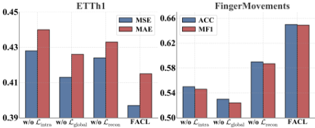
Objective Components. We then examine the contribution of each loss term in FACL's training objective. Figure 3 reports the results of removing each component individually: the global contrastive loss (Lglobal), the intra-subspace contrastive loss (Lintra), and the reconstruction loss (Lrec). Excluding any of these losses causes a clear drop in performance, confirming that each serves a distinct and complementary purpose: Lglobal enforces overall consistency across views, Lintra aligns representations within frequency-specific subspaces, and Lrec preserves essential information by preventing over-attenuation during view construction.
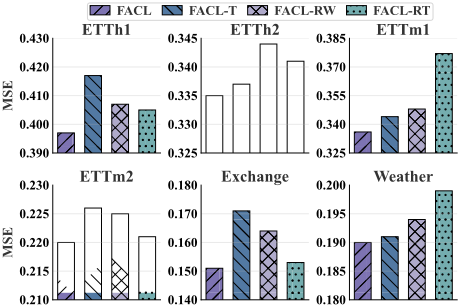
Attenuation Network Analysis To assess the effect of attenuation domain and strategy, we compare three variants: (1) FACL-T, which applies attenuation network in the time domain; (2) FACL-RW, which replaces the learned waveletdomain policy with random attenuation; and (3) FACL-RT, which applies random attenuation in the time domain. All variants are trained under identical settings with prediction length T = 168, and MSE is reported on six datasets. Figure 4 shows that FACL consistently achieves the lowest MSE, reducing error by 3.4% on average compared to FACL-T. Random attenuation harms performance in both domains, with FACL outperforming FACL-RT and FACL-RW by 4.0% and 3.1%, respectively. FACL-T's mixed results over FACLRW suggest that time-domain learning yields only limited and unstable benefits.
4.4 Sensitivity Analysis
We conduct a sensitivity analysis on the weighting coefficients α and β, which regulate the relative contributions of the intra-subspace contrastive loss and the reconstruction loss in the overall training objective.
Effect of α. Figure 5 (a) and (c) illustrate the impact of α on ETTh1 and FingerMovements. For ETTh1, with β = 0.1, MSE decreases from 0.427 at α = 0.001 to a minimum of 0.397 at α = 0.5, and then rises to 0.412 at α = 10. For FingerMovements, with β = 0.5, ACC improves from 55.0% at α = 0.1 to 65.0% at α = 10, and then drops to 51.0% at α = 100. These results suggest that a moderate weight on frequency-level alignment (α between 0.5 and 10) supports both forecasting and classification, while excessively large values distort the objective and harm performance.
Effect of β. Figure 5 (b) and (d) show the effect of β with α fixed (α = 0.5 for ETTh1 and α = 10 for FingerMovements). On ETTh1, MSE reaches its lowest value of 0.397 at β = 0.1. On FingerMovements, ACC rises steadily to 65.0% at β = 0.5 and declines when β exceeds 1. These results indicate that a moderate reconstruction weight helps preserve useful temporal details and complements the contrastive objective, while excessive emphasis (β ≥ 1) disrupts alignment and reduces performance.

4.5 Semi-Supervised Learning
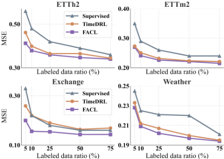
To evaluate performance under limited labeled data, a semisupervised fine-tuning protocol is used. The encoder is first self-supervised on the full unlabeled dataset, then the network is fine-tuned with labeled subsets of 75%, 50%, 25%, 10%, and 5%. For the forecasting experiments in this section, the prediction length is fixed at 168 for all datasets. PatchTST [Nie et al., 2022] is selected as the supervised learning baseline for comparison. Figure 6 shows forecasting error for different labeled percentages on four datasets. Across all label settings, FACL matches or outperforms the strongest baseline, TimeDRL. The performance gap is especially pronounced in low-label scenarios. At the lowest label ratio (5%), FACL maintains a clear advantage over TimeDRL and the supervised baseline. As the proportion of labeled data increases, this advantage gradually narrows, but FACL still achieves lower forecasting error even at higher label ratios. These results demonstrate that FACL makes effective use of unlabeled time series data in semi-supervised settings.
5 RelatedWork
Time Series Contrastive Learning. Contrastive learning has been widely used for time-series representation learning [Zheng et al., 2023; Sharma et al., 2020; Meng et al., 2023; Cheng et al., 2026; Dong et al., 2023; Liu et al., 2024; Zhou et al., 2024]. Early work [Franceschi et al., 2019]
learns embeddings with subsequence triplets, and CPC [Oord et al., 2018] trains an encoder to predict future segments in latent space. TNC [Tonekaboni et al., 2021] uses a debiased contrastive loss. TS-TCC [Eldele et al., 2021] learns through temporal and contextual contrasts. TF-C [Zhang et al., 2022] exploits time-frequency contrastive objective. TS2Vec [Yue et al., 2022] learns representations via hierarchical contrastive objectives. CoST [Woo et al., 2022] applies contrastive learning to capture disentangled seasonal-trend representations, while MF-CLR [Duan et al., 2024] adopts a hierarchical approach to handle multi-rate data heterogeneity. In contrast to MF-CLR, our work addresses the augmentation distortion by leveraging wavelet subspaces. Moreover, despite recent efforts [Chen et al., 2023; Wu et al., 2024; Fu and Hu, 2025] to incorporate frequency-domain information, its potential remains underutilized, especially regarding the structured nature of frequency components.
Adaptive Augmentations. Naive data augmentations for time series often distort the patterns of the data, calling for adaptive augmentation strategies. Prior work includes InfoTS [Luo et al., 2023], which selects augmentations using a meta-learner, and AutoTCL [Zheng et al., 2024], which applies parameterized transformations. Moreover, TimeDRL [Chang et al., 2024] synthesizes views via stochastic dropout to reduce augmentation dependence. SAURL [Liu et al., 2026] proposes a self-adaptive data augmentation module that learns dataset-specific transformations across time and frequency domains. FACL instead introduces a frequencystructured view construction mechanism that leverages the inherent structure of the frequency domain to perform augmentations in an explicit and controlled manner.
6 Conclusion
We proposed FACL, a frequency-aware contrastive learning framework that tackles the limitations of random timedomain augmentations and global-only alignment. FACL employs a frequency-structured view construction mechanism to generate controlled and interpretable views that preserve specific frequency components, and incorporates a multi-level contrastive objective with frequency subspace alignment to capture patterns at multiple scales. Extensive experiments across forecasting and classification tasks show that FACL learns robust representations with consistently strong performance. Future work may investigate adaptive frequency partitioning via learnable filters and develop enriched frequency objectives, further advancing frequency-aware selfsupervised learning for complex temporal data.
Acknowledgments
This work was supported by the Marie Skłodowska-Curie Postdoctoral Individual Fellowship (Grant No. 101154277), the RE-INTEGRATE project funded by the European Union's Horizon Europe Research and Innovation Programme (Grant No. 101118217), the China Scholarship Council (Grant No. 202208410132), and the Fujian Provincial Artificial Intelligence Industry Development Technology Project (Grant No. 2025H0042).
@inproceedings{ijcai2026p320,
  title     = {Frequency-Aware Augmentation and Alignment for Time Series Contrastive Learning},
  author    = {Liu, Yusen and Lai, Zhichen and Lu, Hua and Cheng, Xu and Liu, Xiufeng and Huo, Huan},
  booktitle = {Proceedings of the Thirty-Fifth International Joint Conference on
               Artificial Intelligence, {IJCAI-26}},
  publisher = {International Joint Conferences on Artificial Intelligence Organization},
  editor    = {Diego Calvanese},
  pages     = {2879--2887},
  year      = {2026},
  month     = {8},
  note      = {Main Track},
  doi       = {10.24963/ijcai.2026/320},
  url       = {https://doi.org/10.24963/ijcai.2026/320},
}
TY - CPAPER TI - Frequency-Aware Augmentation and Alignment for Time Series Contrastive Learning AU - Liu, Yusen AU - Lai, Zhichen AU - Lu, Hua AU - Cheng, Xu AU - Liu, Xiufeng AU - Huo, Huan T2 - Proceedings of the Thirty-Fifth International Joint Conference on Artificial Intelligence, IJCAI-26 PB - International Joint Conferences on Artificial Intelligence Organization PY - 2026 SP - 2879 EP - 2887 DO - 10.24963/ijcai.2026/320 UR - https://doi.org/10.24963/ijcai.2026/320 ER -Copied
Machine-readable versions of this paper, for tools and AI agents:





