
Modeling Dynamic Mixtures of Time-Delay Systems from Streaming Time Series
Proceedings of the Thirty-Fifth International Joint Conference on Artificial Intelligence. Main Track. Pages 2617-2625.
https://doi.org/10.24963/ijcai.2026/291
© 2026 International Joint Conferences on Artificial Intelligence
Keywords
- Data Mining: Mining spatial and/or temporal data
- Data Mining: Theoretical foundations of data mining
- Data Mining: Mining data streams
Abstract
This research addresses the problem of adaptive modeling in time-series data streams with clear input-output relationships. This problem is challenging because rapid system changes (regime shifts) caused by environmental factors or input delay changes degrade model performance, and the trade-off among accuracy, robustness, and memory usage arises when using multiple small models for each time-series pattern. To address these issues, this paper presents an online framework/method that treats streaming time series as dynamic mixtures of time-delay systems. This framework maintains robustness of model tracking and reduces memory usage by summarizing past regimes using a fixed-length representation that captures both the system dynamics and input-output delays. Concretely, this approach constructs a summary system tensor using the system's Markov parameter series, capturing both dynamic behavior and delay characteristics. If necessary, a tensor decomposition algorithm extracts relevant past models from the tensor and helps select the system that best fits the current regime. This method enables rapid adaptation to environmental changes and is computationally efficient. Tests on real datasets show that DelayMix consistently outperforms other methods, achieving superior forecast accuracy and faster adaptation to delays, especially for highly non-stationary data.
- [Baeza-Yates et al., 2024] Ricardo Baeza-Yates, Francesco Bonchi, Xihao Piao, Zheng Chen, Taichi Murayama, Ya- suko Matsubara, and Yasushi Sakurai. Fredformer: Fre- quency debiased transformer for time series forecasting. In Proceedings of the 30th ACM SIGKDD Conference on Knowledge Discovery and Data Mining, pages 2400- 2410, 2024.
- [Baier and Staab, 2022] Alexandra Baier and Steffen Staab. A simulated 4-DOF ship motion dataset for system identi- fication under environmental disturbances, 2022.
- [Baier et al., 2023] Alexandra Baier, Decky Aspandi, and Steffen Staab. ReLiNet: Stable and explainable mul- tistep prediction with recurrent linear parameter varying networks. In Proceedings of the Thirty-Second Interna- tional Joint Conference on Artificial Intelligence, pages 3461-3469, 2023. IJCAI
- [Bakshi et al., 2023] Ainesh Bakshi, Allen Liu, Ankur Moitra, and Morris Yau. Tensor decompositions meet con- trol theory: Learning general mixtures of linear dynamical systems. In International Conference on Machine Learn- ing, volume 202 of Proceedings of Machine Learning Re- search, pages 1549-1563, 2023.
- [Bertsimas and Gurnee, 2023] Dimitris Bertsimas and Wes Gurnee. Learning sparse nonlinear dynamics via mixed- integer optimization. Nonlinear Dynamics, 111(7):6585- 6604, 2023.
- [Box and Jenkins, 1968] George E. P. Box and Gwilym M. Jenkins. Some recent advances in forecasting and control. Journal of the Royal Statistical Society. Series C (Applied Statistics), 17(2):91-109, 1968.
- [Box and Tiao, 1975] George E.P. Box and George C. Tiao. Intervention analysis with applications to economic and environmental problems. Journal of the American Statis- tical Association, 70(349):70-79, 1975.
- [Brunton et al., 2016a] Steven L Brunton, Joshua L Proctor, and José Nathan Kutz. Discovering governing equations from data by sparse identification of nonlinear dynamical systems. Proceedings of the national academy of sciences, 113(15):3932-3937, 2016.
- [Brunton et al., 2016b] Steven L. Brunton, Joshua L. Proc- tor, and José Nathan Kutz. Sparse identification of nonlinear dynamics with control (SINDYc). IFAC- PapersOnLine, 49(18):710-715, 2016. 10th IFAC Sym- posium on Nonlinear Control Systems NOLCOS 2016.
- [Chen and Poor, 2022] Yanxi Chen and H Vincent Poor. Learning mixtures of linear dynamical systems. In Inter- national Conference on Machine Learning, volume 162 of Proceedings of Machine Learning Research, pages 3507- 3557, 2022.
- [Chihara et al., 2025] Naoki Chihara, Yasuko Matsubara, Ren Fujiwara, and Yasushi Sakurai. Modeling time- evolving causality over data streams. Proceedings of the 31st ACM SIGKDD Conference on Knowledge Discovery and Data Mining V.1, pages 153-164, 2025.
- [Fawaz et al., 2019] Hassan Ismail Fawaz, Germain Forestier, Jonathan Weber, Lhassane Idoumghar, and Pierre-Alain Muller. Deep learning for time series classifi- cation: a review. Data Mining and Knowledge Discovery, 33:917-963, 2019.
- [Folke et al., 2004] Carl Folke, Steve Carpenter, Brian Walker, Marten Scheffer, Thomas Elmqvist, Lance Gun- derson, and C.S. Holling. REGIME SHIFTS, RE- SILIENCE, AND BIODIVERSITY IN ECOSYSTEM MANAGEMENT. Annual Review of Ecology, Evolution, and Systematics, 35:557-581, 2004.
- [Fujiwara et al., 2025] Ren Fujiwara, Yasuko Matsubara, and Yasushi Sakurai. Modeling latent non-linear dynami- cal system over time series. Proceedings of the AAAI Con- ference on Artificial Intelligence, 39(11):11663-11671, 2025.
- [García et al., 1989] Carlos E. García, David M. Prett, and Manfred Morari. Model predictive control: Theory and practice-a survey. Automatica, 25:335-348, 1989.
- [Gorbach et al., 2017] Nico S. Gorbach, Stefan Bauer, and Joachim M. Buhmann. Scalable variational inference for dynamical systems. In Advances in Neural Information Processing Systems, volume 30, pages 4806-4815, 2017.
- [Gui et al., 2025] Shurui Gui, Xiner Li, and Shuiwang Ji. Discovering physics laws of dynamical systems via invari- ant function learning. In Forty-second International Con- ference on Machine Learning, 2025.
- [Hare and Mantua, 2000] Steven R Hare and Nathan J Man- tua. Empirical evidence for north pacific regime shifts in 1977 and 1989. Progress in Oceanography, 47:103-145, 2000.
- [Heinonen et al., 2018] Markus Heinonen, Cagatay Yildiz, Henrik Mannerström, Jukka Intosalmi, and Harri Lähdesmäki. Learning unknown ODE models with Gaussian processes. In International Conference on Machine Learning, volume 80, pages 1959-1968.
- PMLR, 2018.
- [HO and Kalman, 1966] Bin-Lun HO and Rudolf E. Kalman. Editorial: Effective construction of linear state-variable models from input/output functions. auto, 14(1-12):545-548, 1966.
- [Kalman, 1963] Rudolf E. Kalman. Mathematical descrip- tion of linear dynamical systems, volume 1. 1963.
- [Lauer, 2013] Fabien Lauer. Estimating the probability of success of a simple algorithm for switched linear regres- sion. Nonlinear Analysis: Hybrid Systems, 8:31-47, 2013.
- [Lazic et al., 2018] Nevena Lazic, Craig Boutilier, Tyler Lu, Eehern Wong, Binz Roy, MK Ryu, and Greg Imwalle. Data center cooling using model-predictive control. Ad- vances in Neural Information Processing Systems, 2018.
- [Li et al., 2009] Lei Li, James McCann, Nancy S Pollard, and Christos Faloutsos. DynaMMo mining and summa- rization of coevolving sequences with missing values. In Proceedings of the 15th ACM SIGKDD international con- ference on Knowledge discovery and data mining, pages 507-516, 2009.
- [Li et al., 2022] Ming-Wei Li, Dong-Yang Xu, Jing Geng, and Wei-Chiang Hong. A hybrid approach for forecast- ing ship motion using cnn-gru-am and gcwoa. Applied Soft Computing, 114, 2022.
- [Lu et al., 2021] Haodong Lu, Miao Du, Kai Qian, Xiaom- ing He, and Kun Wang. Gan-based data augmentation strategy for sensor anomaly detection in industrial robots. IEEE Sensors Journal, pages 17464-17474, 2021.
- [Luo et al., 2022] Yingtao Luo, Chang Xu, Yang Liu, Weiqing Liu, Shun Zheng, and Jiang Bian. Learning dif- ferential operators for interpretable time series modeling. In Proceedings of the 28th ACM SIGKDD Conference on Knowledge Discovery and Data Mining, KDD '22, page 1192-1201, New York, NY, USA, 2022. Association for Computing Machinery.
- [Matsubara and Sakurai, 2016] Yasuko Matsubara and Ya- sushi Sakurai. Regime shifts in streams real-time forecast- ing of co-evolving time sequences. In Proceedings of the 22th ACM SIGKDD International Conference on Knowl- edge Discovery and Data Mining, pages 1045-1054, 2016.
- [Matsubara and Sakurai, 2025] Yasuko Matsubara and Ya- sushi Sakurai. Microadapt: Self-evolutionary dynamic modeling algorithms for time-evolving data streams. In Proceedings of the 31st ACM SIGKDD Conference on Knowledge Discovery and Data Mining V.2, KDD '25, page 2114-2125, New York, NY, USA, 2025. Association for Computing Machinery.
- [Nie et al., 2023] Yuqi Nie, Nam H Nguyen, Phanwadee Sinthong, and Jayant Kalagnanam. A time series is worth 64 words: Long-term forecasting with transformers. In The Eleventh International Conference on Learning Rep- resentations, 2023.
- [Ortner and del Re, 2007] Peter Ortner and Luigi del Re. Predictive control of a diesel engine air path. IEEE Trans- actions on Control Systems Technology, 2007.
- [Park et al., 2025] Hyuk Park, Grani A. Hanasusanto, and Yingying Li. Robust system identification: Finite-sample guarantees and connection to regularization. In The Thir- teenth International Conference on Learning Representa- tions, 2025.
- [Proctor et al., 2016] Joshua L. Proctor, Steven L. Brunton, and José Nathan Kutz. Dynamic mode decomposition with control. SIAM Journal on Applied Dynamical Systems, 15(1):142-161, 2016.
- [Punjani and Abbeel, 2015] Ali Punjani and Pieter Abbeel. Deep learning helicopter dynamics models. 2015 IEEE International Conference on Robotics and Automation (ICRA), pages 3223-3230, 2015.
- [Salinas et al., 2017] David Salinas, Valentin Flunkert, and Jan Gasthaus. DeepAR: Probabilistic forecasting with au- toregressive recurrent networks. International journal of forecasting, 36:1181-1191, 2017.
- [Scheffer et al., 2001] Marten Scheffer, Steve Carpenter, Jonathan A. Foley, Carl Folke, and Brian Walker. Catas- trophic shifts in ecosystems. Nature, 413:591-596, 2001.
- [Tajeuna et al., 2023] Etienne Gael Tajeuna, Mohamed Bouguessa, and Shengrui Wang. Modeling regime shifts in multiple time series. ACM Trans. Knowl. Discov. Data, 17(8), June 2023.
- [Wang et al., 2024] Yuxuan Wang, Haixu Wu, Jiaxiang Dong, Guo Qin, Haoran Zhang, Yong Liu, Yunzhong Qiu, Jianmin Wang, and Mingsheng Long. TimeXer: Empow- ering transformers for time series forecasting with exoge- nous variables. In Advances in Neural Information Pro- cessing Systems 37, 2024.
- [Weigand et al., 2022] Jonas Weigand, Julian Götz, Jonas Ulmen, and Martin Ruskowski. Dataset and baseline for an industrial robot identification benchmark, 2022.
- [Williams et al., 2016] Grady Williams, Paul Drews, Brian Goldfain, James M. Rehg, and Evangelos A. Theodorou. Aggressive driving with model predictive path integral control. In 2016 IEEE International Conference on Robotics and Automation, ICRA 2016, Stockholm, Swe- den, May 16-21, 2016, 2016.
- [Zeng et al., 2023] Ailing Zeng, Muxi Chen, Lei Zhang, and Qiang Xu. Are transformers effective for time series fore- casting? In Proceedings of the AAAI Conference on Arti- ficial Intelligence, volume 37, pages 11121-11128, 2023.
- [Zhou et al., 2020] Haoyi Zhou, Shanghang Zhang, Jieqi Peng, Shuai Zhang, Jianxin Li, Hui Xiong, and Wancai Zhang. Informer: Beyond efficient transformer for long sequence time-series forecasting. In Proceedings of the AAAI Conference on Artificial Intelligence, volume 35, pages 11106-11115, 2020.
References were extracted automatically from the PDF and may contain errors.
Full text extracted automatically from the PDF; figures, tables and equations may differ. The PDF is the version of record.
1 Introduction
In recent years, the importance of modeling time-series data streams with explicit input-output relationships and modeling based on such data streams has grown. In particular, in real-world systems such as ship control [Li et al., 2022], industrial robots [Lu et al., 2021], data center cooling [Lazic et al., 2018], diesel engine control [Ortner and del Re, 2007], and autonomous driving [Williams et al., 2016], modeling failures can easily manifest as failures in safe and efficient operation, necessitating the development of methods for stable and efficient modeling on time-series data streams.
However, modeling on streams simultaneously faces the challenges of data nonstationarity and computational resource constraints, making it difficult to directly apply models and algorithms designed for offline use. Specifically, the following two problems arise: (1) Changes in the underlying system often cause abrupt model changes, or regime shifts, rapidly degrading the performance of trained models [Folke et al., 2004; Hare and Mantua, 2000; Scheffer et al., 2001]. Furthermore, this challenge is further complicated by the unknown input delay inherent in systems with input-output relationships [Box and Tiao, 1975; Garc´ıa et al., 1989; Lauer, 2013; Punjani and Abbeel, 2015; Brunton et al., 2016b; Proctor et al., 2016; Baier et al., 2023]. This means that changes in the model's input delays must be simultaneously tracked. (2) Time-series data streams have no temporal boundaries (i.e., they are semi-infinitely long), making model estimation using all past data prone to design errors. Furthermore, models designed using multiple small models for each time-series pattern suffer from a trade-off between robustness of accuracy and memory usage. While retaining more models stabilizes accuracy, having too many models increases the model search cost and memory computational complexity without bound.
For example, current stream prediction models that consider regime shifts offer scalable algorithms in terms of model adaptability and computational time on the stream [Matsubara and Sakurai, 2016; Tajeuna et al., 2023; Chihara et al., 2025; Matsubara and Sakurai, 2025]. However, these methods monotonically increase the number of models, thereby increasing not only memory usage but also the computational time required for model switching. Furthermore, these methods do not consider exogenous variables. In other words, these methods lack design principles for tracking changes in input delay, making them difficult to directly apply to our problem. Recent neural approaches, such as ReLiNet [Baier et al., 2023] and TimeXer [Wang et al., 2024], incorporate exogenous signals through switched linear systems and Transformer-based attention, respectively, achieving competitive results. However, these models generally do not model time delays explicitly and tend to struggle in streaming settings due to high computational cost and frequent retraining. Therefore, this paper aims to develop a method that simultaneously satisfies both adaptability to sudden environmental changes and scalable estimation. The research question in this paper is:
Can we develop a method that achieves high-accuracy modeling of time-series data streams with explicit inputoutput relationships, while tracking rapid environmental changes and maintaining high computational efficiency?
We propose DelayMix, an online framework that resolves the conflict between structural identification and streaming adaptation. This framework maintains high model tracking performance while avoiding increased memory usage by retaining model sets used in past regimes as mixtures of fixedlength summarized representations of the system's dynamic behavior and input-output delay structure. Specifically, we focus on the fact that the system's Markov parameter series integrates its dynamic behavior and input-output delay structure, and we construct a system tensor that summarizes them. Then, if necessary, we use a tensor decomposition algorithm to extract useful past models from the system tensor and adaptively select the system that best fits the current regime. This approach achieves both tracking rapid environmental changes and high computational efficiency.
In summary, DelayMix is an online algorithm for modeling streaming time series as mixtures of time-delay systems. Our main contributions are as follows:
- StreamingModeling of Time-Delay Systems: We propose a new formulation that leverages Markov parameter sequences to jointly learn unknown delays and system dynamics in streaming environments.
- Scalability with Resource Constraints: The computation time of DelayMix is independent of the time series length, thanks to incremental model updating, and thus is a faster algorithm than its competitors.
- Robustness Against Structural Drift: Experiments on real-world datasets demonstrate that our method significantly outperforms state-of-the-art baselines in predictive accuracy, especially in environments with strong nonstationarity.
2 ProposedMethod
In this paper, we study time series arising from mixtures of time-delay MIMO systems, where the delays are unknown and may differ across systems. Our goal is to recover the dynamics of each system from one observed sequence and use them for online multi-step forecasting. Rather than estimating delays directly, we estimate Markov parameters for each regime to summarize input-output behavior. For each regime, we then create a delay-free input-output equivalent state-space model, which we use for inference and prediction.
This section introduces the proposed model and the algorithm. First, in section 2.1, we define our model. Then we formalize the problem definition in Problem 1. We then present the proposed online algorithm DelayMix, which includes sub-algorithms named DynamicMomentCollection, ModelDatabaseAdaption, and FuturePrediction. The theoretical justification for our method is given in Section 3.
2.1 Mixtures of Time-Delay Systems
In practice, time-series data rarely come from just one stationary dynamical system. Instead, the underlying dynamics often switch between several regimes, depending on hidden conditions such as the operating mode, environment, or user behavior. To capture this non-stationarity, we model the data as coming from a mixture of time-delay systems.
Let R denote the number of regimes, and let rt → ¶1↪ ▷ ▷ ▷ ↪R♦ denote the (unobserved) regime index at time t. For each regime i → ¶1↪ ▷ ▷ ▷ ↪R♦, we introduce a latent state zi(t) → Rk and system matrices Ai → Rk→k ↪Bi → Rk→dc ↪ Ci → Rd→k ▷ We also include an integer-valued delay ωi ↑ 0 in the state update. Conditioned on being in regime rt = i at time t, the dynamics evolve as
where u(t) → Rdc is the observed exogenous input and x(t) → Rd is the observed output. The input u(t) is observed at every time step, but the regime index rt and the latent states zi(t) are not directly observed. We use ˆx(t) for model predictions (for example, predictions produced by filtering) when needed later.
Regime-specific Markov parameters and mixture view. For each regime, the time-delay system (1)-(2) yields the following equivalent Markov parameters (impulse response):
When an explicit delay ωi exists in the system, the Markov parameters exhibit a characteristic pattern: in the ideal noisefree case, the first ωi Markov parameters vanish, and nonzero responses begin at delay ωi + 1. This relationship between the Markov parameters and the time delay suggests that simply estimating the Markov parameters, without explicitly accounting for the delay, yields an estimate of the time-delay system. Furthermore, estimating the regimes represented by the time-delay system can be reformulated as the problem of estimating mixtures of Markov parameters from the data. Here, in [Bakshi et al., 2023], it was theoretically shown that mixtures of Markov parameters in observed data can be extracted by decomposing a properly generated third-order tensor (i.e., the system tensor) as a superposition of rank-1 tensors. In this work, we construct an algorithm that applies this theoretical framework to regime estimation for time-delay systems in real-world streaming settings. In the rest of this section, we focus on the proposed algorithm.
2.2 Online Forecasting withMoment-Based System Tensors
We now explain how DelayMix uses moment-based system tensors for online modeling and the main idea is to keep an up-to-date empirical estimate of a system tensor at each update that summarizes the higher-order moments of (x↪ u), and to periodically factorize this tensor to update a mixture of delay-free state-space models. We then use these models to infer the current dynamical regime and to forecast future outputs based on the exogenous inputs.
Data Windows and Exogenous Variables
We assume that the data stream X, denoted as ¶x(t)♦t↓1, arrives sequentially. The algorithm runs at set update times, processing a sliding window of the most recent data.
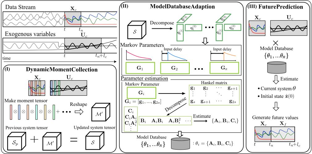
Definition 1 (Current data window: Xc ). Let Xc = X[t : tn] denote the subsequence of length lc extracted from the observed time series, starting at time index t and ending at tn.
Definition 2 (Current exogenous variables: Uc ). Let Uc = U[t : tn + ls] denote the subsequence of exogenous inputs available at the current update, where ls is the forecasting horizon. The segment U[t : tn] is used for updating the model, and U[tn + 1 : tn + ls] is used for forecasting.
We focus on modeling streaming data as a mixture of timedelay systems and on using dynamics for forecasting, which is one of the primary applications of DelayMix. At each update, the algorithm observes the current data windowXc and the corresponding exogenous input sequence Uc , along with the model estimated up to the previous update. With this information, our goal is to refine the current systemmixture and predict the ls-step-ahead outputs.
We formalize the problem as follows.
Problem 1. Given the current data window Xc , the exogenous input sequence Uc sampled at regular time intervals, the previously estimated model parameters εp, and the previous system tensor Sp, at each update do the following:
- Update the system tensor S and the current system parameters
to better fit the newly observed data;
- Predict the future outputs Xf = X[tn + 1 : tn + ls] given the future inputs U[tn + 1 : tn + ls];
- Maintain computational efficiency and bounded memory usage as new data arrives.
To solve Problem 1, DelayMix organizes the online estimation and forecasting pipeline into three parts: DynamicMomentCollection (system tensor collection), ModelDatabaseAdaption (online model adaptation via tensor factorization and system realization), and FuturePrediction (forecasting trajectories with the delay-free models). We describe each part in turn. Figure 1 shows an overview of DelayMix, from the current data window and exogenous inputs to the updated models and forecasts.
The goal of DynamicMomentCollection is to maintain an up-to-date empirical estimate of the global system tensor S using streaming input-output data. We build structured higher-order moments to capture the temporal dependencies from the underlying switching dynamical systems. Our approach uses a compact method inspired by [Bakshi et al., 2023] that does not require storing raw data. DynamicMomentCollection keeps running estimates of the necessary moment blocks and updates S incrementally as new samples arrive. This keeps memory usage low while preserving a tensor whose CP decomposition can recover the regime-specific Markov parameters, up to scaling and permutation. Concretely, for a sub-window start time ω and a triplet (k1↪ k2↪ k3) → ¶1↪ ▷ ▷ ▷ ↪ kmax♦3 , define
t1 = ω + k1↪ t2 = ω + k1 + k2 + 1↪ t3 = ω + k1 + k2 + k3 + 2↪ ˜ t1 = ω↪ ˜ t2 = ω + k1 + 1↪ ˜ t3 = ω + k1 + k2 + 2▷ Using these indices, we form empirical sixth-order moments over three output-input pairs and, for computational efficiency, we group each pair into a single mode using vec(x(tj)u(tj)↔)(j = 1↪ 2↪ 3), yielding a third-order moment block M↗ (k1↪ k2↪ k3) → Rp→p→p . We combine these blocks across valid ω and triplets to form the system tensor S using an incremental update.
ModelDatabaseAdaption: Online Model Adaptation via Tensor Factorization
The goal of ModelDatabaseAdaption is to find and update the set of dynamical systems ε from a moment-based tensor representation. While DynamicMomentCollection keeps updating S, extracting separate system modes requires a more involved tensor decomposition and system realization step. This step is triggered only when a change in dynamics is detected or when enough new data have been collected.
The adaptation procedure has the following steps:
- Tensor decomposition: We apply the Alternating Least Squares (ALS) algorithm to the system tensor S to approximate it by a rank-R CP decomposition
where (q(1) i ↪ q(2) i ↪ q(3) i ) are factor vectors associated with component i. Under the assumptions stated in Theorem 2, the rank-one components can be associated with individual regimes and their stacked Markov parameters.
- Markov parameter reconstruction and delay-free realization: For each component i, we rearrange the factor vectors (q(1) i ↪ q(2) i ↪ q(3) i ) into a sequence of estimated Markov parameters ¶ˆg(i) k ♦Kk=1 by following the construction of the system tensor (see also Section 3). The initial zero pattern in this sequence implicitly encodes the effective delay for regime i, but we do not explicitly estimate the delay. Instead, we treat ¶ˆg(i) k ♦ as the Markov parameters of an input-output equivalent system and apply a standard realization procedure, such as the Ho-Kalman algorithm [HO and Kalman, 1966] to obtain a delay-free state-space model:
By Theorem 1 in Section 3, the resulting delay-free model ¶Ai↪Bi↪Ci♦ is input-output equivalent to a time-delay system and thus it faithfully captures the behavior of regime i. Finally, these parameters can be optionally fine-tuned so as to better fit the current data Xc , and the collection of all such systems constitutes the updated set ε.
In summary, ModelDatabaseAdaption uses tensor factorization to separate regime-specific Markov parameters from the system tensor and then realizes, for each regime, a delayfree state-space model that is suitable for inference and forecasting.
FuturePrediction: Forecasting Trajectories with Delay-Free Models
The goal of FuturePrediction is to infer a suitable initial state for the currently active system and use it, together with the learned models, to generate future values. Given the updated set of delay-free systems ε and the current data window (Xc ↪Uc ), we first infer the active regime and its latent states, for example, by running a bank of Kalman filters and smoothers, one per regime. We utilize the forward-pass (filter) and backward-pass (smoother) equations.
The backward pass gives a smoothed estimate of the state trajectory, including an estimate of the current (or initial) state ˆz(0) for the active delay-free system. Using this state estimate and the identified system matrices ¶Ai↪Bi↪Ci♦, we then simulate the delay-free dynamics forward in time, using the future inputs U[tn + 1 : tn + ls], to generate the ls-stepahead future values Xf .
By Theorem 1, each delay-free model ¶Ai↪Bi↪Ci♦ obtained in this way is input-output equivalent to a time-delay system representing regime i. This means forecasting with these delay-free models is theoretically justified.
3 Theoretical Analysis
In this section, we explain the theoretical foundations behind the modeling approach. We also discuss the assumptions and algorithmic design choices introduced earlier. We focus on two main components that are central to DelayMix. First, we represent each time-delay MIMO system, which corresponds to one regime in the mixture model, using a delayfree state-space model built from its Markov parameters. Second, we recover the regime-specific Markov parameters from a moment-based system tensor using CP decomposition. We then analyze the computational complexity of the online algorithm DelayMix.
3.1 Equivalence of a Time-Delay System to a Standard MIMO Model
We begin by formalizing the relationship between a timedelay MIMO system and an equivalent delay-free state-space model. Recall from Section 2.1 that each regime i in the mixture model is described by a time-delay MIMO system. For clarity, we first focus on a single system and drop the regime index i. The equivalence result in this subsection supports the realization step in ModelDatabaseAdaption and the forecasting step FuturePrediction in DelayMix.
Consider a single segment of a time-delay system described by
where ω ↑ 0 represents an explicit delay in the state update, A↗ → Rk→k governs the latent dynamics, B↗ → Rk→dc captures the influence of the delayed input u(t ↓ ω), and C↗ → Rd→k maps the latent state to the observation. For simplicity, we do not include direct-feedthrough terms or additive noise.
The Markov parameters of this delayed system are defined by its impulse response to an input that is zero everywhere except at a single time step. They are given by
The first ω zeros represent the delay, while the subsequent nonzero entries characterize the response after the delay. It is well known that there exists a delay-free state-space realization whose Markov parameters match this sequence. In other words, the explicit delay can be included in an augmented state.
The next theorem shows that any minimal delay-free realization with matching Markov parameters is input-output equivalent to the original delayed system.
Theorem 1. Suppose that the delayed system (3)-(4) is minimal (reachable and observable). Let (A↪ B↪ C) be any minimal delay-free state-space realization whose Markov parameters ¶CAj↑1B♦j↓1 coincide with those of the delayed system. Then the delayed and delay-free systems are inputoutput equivalent: for any input sequence and any initial state of the delayed system, there exists a corresponding initial state of the delay-free realization such that the resulting output sequences coincide.
Proof sketch of Theorem 1. The claim follows from the standard augmented-state construction. Define an augmented state that contains the original latent state and a buffer of the past ω inputs. The augmented transition matrix updates the original state using the oldest buffered input, shifts the buffer by one step, and inserts the current input into the buffer. This gives a delay-free state-space realization. By construction, its first ω Markov parameters are zero and the remaining Markov parameters coincide with those of the delayed system. Therefore, for any input sequence, the two systems have the same input-output behavior under corresponding initial states.
Theorem 1 simplifies the problem of identifying a delayed system to estimating its possibly sparse sequence of Markov parameters from data. This supports working in the standard state-space framework without explicitly modeling delays, as long as the Markov parameters are correctly captured. In particular, this supports the modeling choice in DelayMix to perform inference forecasting entirely in terms of delay-free state-space models realized from estimated Markov parameters.
3.2 Moment Tensor Representation and Tensor Factorization
Next, we summarize the moment-based tensor representation used in the online estimation algorithm of DelayMix. In the previous section, we introduced the system tensor S as a compact way to encode higher-order moments of the input-output data and as the object for CP decomposition in DynamicMomentCollection and ModelDatabaseAdaption. Here we state a concise result from [Bakshi et al., 2023], which shows that factorizing a properly constructed moment tensor is enough to recover the Markov parameters of the underlying systems.
Theorem 2 (Recovery of Markov parameters via moment tensor factorization [Bakshi et al., 2023]). Let (u(t)↪ x(t))t↓1 be generated by a (mixture of) linear timedelay MIMO systems with regime-specific Markov parameters ¶h(i) j ♦j↓1. Assume that the exogenous inputs are independent and identically distributed, with a distribution that satisfies suitable moment conditions, and that the resulting moment tensor is well-defined. Then there exists a polynomial-time procedure that constructs a tensor S from empirical moments of (u(t)↪ x(t)) such that, under mild identifiability conditions, any sufficiently accurate CP decomposition of S recovers the Markov parameters ¶h(i) j ♦j↓1 of the constituent systems, up to permutation and scaling of the components.
Proof. See [Bakshi et al., 2023] for the complete proof.
This theorem gives the theoretical justification for the tensor factorization step in DelayMix. The CP factors obtained by applying ALS to the empirical system tensor in ModelDatabaseAdaption can be seen as estimates of the regimespecific Markov parameters. Combined with Theorem 1, this ensures that the subsequent realization step produces delayfree models whose input-output behavior matches that of the underlying time-delay systems.
3.3 Computational Complexity of DelayMix
Finally, we analyze the computational complexity of the proposed online algorithm DelayMix. The dominant computational cost arises from the ALS-based tensor decomposition used to update the system tensor representation, along with the following realization of state-space models.
LEMMA 1 (Time complexity of DelayMix). Given a new incoming tensor (i.e., an updated system tensor S), the time complexity of one update of DelayMix is
where i is the number of ALS iterations for tensor decomposition, s is the maximum lag used to construct S, R is the CP rank, lc is the length of the current data window, and ls is the forecasting horizon.
Proof sketch of Lemma 1. Let p = 2sddc be the mode size of the constructed third-order system tensor. One ALS iteration for a rank-R CP decomposition costs O(p3R+pR2 ), and repeating it for i iterations gives the first term. The remaining terms are the costs of state inference on the current window and simulation over the forecasting horizon.
The computational cost of DelayMix mainly depends on the ALS-based tensor decomposition, especially on the number of iterations i needed for convergence. To reduce this cost in practice, the full decomposition step is only triggered when there is a significant mismatch between the current model and the newly updated system tensor is detected. This helps avoid unnecessary updates. Also, because the data changes gradually over time, consecutive system tensors are similar. As a result, initializing ALS with the previous factor estimates usually leads to fast convergence (small i). These properties allow DelayMix to work efficiently in streaming settings while maintaining accurate modeling and forecasting performance.
4 Experimental Results
In this section, we describe the performance of DelayMix using real datasets. The experiments were designed to answer the following questions about DelayMix:
Q1.Accuracy: How accurately does it predict future events?
Q2.Scalability: How does it scale in terms of computational time and memory?
4.1 Experimental Setup
Datasets. To evaluate DelayMix, we use three real-world datasets.
For the evaluation of predictive accuracy (Q1) and scalability (Q2), we used the following three publicly available real-world datasets:
- Ship-OOD/Ship-IND [Baier and Staab, 2022] is a 4DOF ship maneuvering dataset under environmental disturbances. The 4 exogenous variables include propeller speed, rudder angles, and wind; outputs are also 4 (linear and angular velocities). We use both indistribution (Ship-IND) and out-of-distribution (ShipOOD) test sets.
- Robot [Weigand et al., 2022] is a dataset of a 6-DOF industrial robot arm, with 6 exogenous inputs (motor torques) and 6 outputs (joint angles).
Baseline Methods. We compare DelayMix with state-of-theart models that explicitly incorporate exogenous variables, including StableReLiNet, ReLiNet [Baier et al., 2023], and TimeXer [Wang et al., 2024]. Many existing forecasting models either omit exogenous inputs or treat them as endogenous, limiting their ability to model structured input-output relationships. Accordingly, we exclude such models from our main comparison.
Hyperparameter Setting of DelayMix. We selected ϑ → ¶0▷5↪ 0▷6↪ 0▷7↪ 0▷8↪ 0▷9↪ 1▷0♦ and R → ¶2↪ 4↪ 8↪ 10♦ using the validation set, and fixed s = 3.
| Method | DelayMix | TimeXer | ReLiNet | StableReLiNet | |||||
|---|---|---|---|---|---|---|---|---|---|
| Dataset | ls | MSE | MAE | MSE | MAE | MSE | MAE | MSE | MAE |
| Ship-OOD | 1 10 30 | 28 26 27 | 26 28 25 | 1 2 0 | 3 1 0 | 0 0 1 | 0 0 1 | 0 1 1 | 0 0 3 |
| Ship-IND | 1 10 30 | 18 16 16 | 9 6 8 | 12 14 13 | 21 24 22 | 0 0 1 | 0 0 0 | 0 0 0 | 0 0 0 |
| Robot | 1 10 30 | 8 7 5 | 7 3 1 | 4 5 0 | 5 9 0 | 0 0 0 | 0 0 0 | 0 0 7 | 0 0 11 |
4.2 Q1: Accuracy
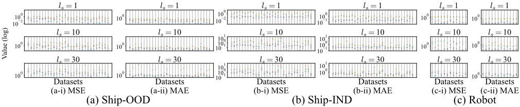
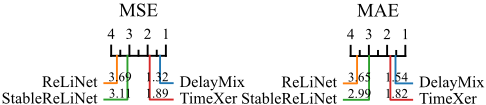
We evaluated DelayMix using mean squared error (MSE) and mean absolute error (MAE), where lower values indicate better accuracy. Results are averaged over five trials for robustness. As shown in Fig. 2, DelayMix consistently yields lower errors than baselines. The critical difference diagram in Fig. 3, based on the Wilcoxon-Holm test [Fawaz et al., 2019], confirms these improvements are statistically significant. Table 1 reports how often each method ranks best, further highlighting the advantage of DelayMix.
A key strength of DelayMix is its ability to adaptively estimate a mixture of time-delay systems in streaming settings, enabling it to capture dynamic and heterogeneous temporal patterns without prior knowledge of delay structures or access to past data. While TimeXer performs well on the stationary Ship-IND dataset, it falls short on the non-stationary ShipOOD data, where adaptive modeling is crucial. In contrast, models like StableReLiNet and ReLiNet tend to degrade under streaming updates, likely due to unstable parameter adaptation. For example, ReLiNet shows noticeably lower accuracy in several scenarios (see Fig. 2). These results show that DelayMix enables accurate real-time prediction in dynamic streaming settings.
4.3 Q2: Scalability
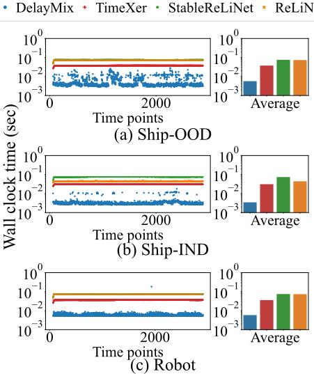
Next, we evaluated the performance of DelayMix in terms of computation time. The left column of Fig. 4 shows the wall clock time of the experiments performed on each dataset. Thanks to an effective parameter estimation algorithm, the computation time of DelayMix is independent of the length of the data stream. Several small spikes are due to the execution of ModelDatabaseAdaption. CP decomposition for updating the regime database increases the computation time for that time step. The right column of Fig. 4 shows the average computation time for the entire tensor stream. Notably, TimeXer and ReLiNet were run in a relatively fast environment, as all computations, including forecasting future values and parameter updating using lightweight single-sample gradients, are performed on the GPU. However, DelayMix is still overwhelmingly faster than them. This demonstrates that DelayMix achieves a high trade-off between accuracy and efficiency.
5 RelatedWork
This section reviews related work on mixtures of dynamical systems and time-series forecasting.
Learning Mixtures of Dynamics. Traditionally, dynamical system estimation has centered on a single system [Brunton et al., 2016a; Gorbach et al., 2017; Heinonen et al., 2018; Luo et al., 2022; Bertsimas and Gurnee, 2023; Fujiwara et al., 2025; Park et al., 2025; Gui et al., 2025], but recent advances enable learning mixed systems-where multiple dynamical regimes coexist-from unlabeled trajectory data. For example, [Chen and Poor, 2022] proposes a spectral algorithm that learns a mixture from short unlabeled trajectories with end-to-end guarantees, and [Bakshi et al., 2023] introduces a tensor-based framework that recovers LDS mixtures via Markov parameters estimated from high-order moments. These approaches are theoretically appealing but inherently offline: constructing the required moment tensors assumes access to the full dataset, which is impractical in streaming scenarios such as industrial process control. Moreover, they handle delays only implicitly and do not explicitly model unknown or time-varying delays, making it difficult to adapt to abrupt changes in system dynamics. DelayMix builds on the framework of [Bakshi et al., 2023] and extends it to streaming data by incrementally updating a system tensor and adaptively estimating multiple time-delay systems from incoming observations.
Time-Series Forecasting Methods. Classical forecasting methods such as ARIMA and Kalman filters [Box and Jenkins, 1968; Kalman, 1963; Li et al., 2009] remain standard tools, and recent deep learning models [Zhou et al., 2020; Salinas et al., 2017; Zeng et al., 2023; Nie et al., 2023; Baeza-Yates et al., 2024] have achieved strong empirical performance. However, many of these methods either ignore exogenous variables or treat them in the same way as endogenous variables, although exogenous inputs often play a distinct and crucial role in prediction. To better exploit exogenous information, ARIMAX [Box and Tiao, 1975] extends ARIMA with exogenous regressors, while recent neural approaches such as ReLiNet [Baier et al., 2023] and TimeXer [Wang et al., 2024] incorporate exogenous signals through switched linear systems and Transformer-based attention, respectively, achieving competitive results. However, these models generally do not model time delays explicitly and tend to struggle in streaming settings due to high computational cost and frequent retraining, whereas DelayMix is designed for online operation: it maintains a compact summary of input-output relationships, explicitly captures delay dynamics, and updates models efficiently in real time.
6 Conclusion
We introduce DelayMix, an online framework for modeling dynamic mixtures of time-delay systems from streaming time series. Our approach addresses key challenges in streaming scenarios, including nonstationarity, unknown delays, and limited resources, while maintaining both accuracy and scalability over long horizons. DelayMix incrementally builds and decomposes high-order moment tensors to extract regimespecific Markov parameter sequences, which efficiently capture system dynamics and input-output delays in a compact, delay-sensitive representation. This allows for delay-aware identification even when regimes switch, without assuming known change points or fixed delay structures. The framework does not require direct access to the system or prior knowledge of delay lengths. Instead, it uses moment-based summaries that are updated online, so it does not need to store the entire history, keeping memory use low and computation efficient. DelayMix can also update its set of candidate systems when the current model no longer fits new observations, helping it adapt to changing dynamics while avoiding unbounded memory growth or switching costs. Our experiments with real-world datasets show that DelayMix consistently achieves better prediction accuracy and computational efficiency than other methods by accurately tracking changing delays and adapting to regime shifts.
Acknowledgements
This work was supported by JSPS KAKENHI Grant-in-Aid for Scientific Research Number JP26H02499, JST CREST JPMJCR23M3, JST K Program JPMJKP25Y6, JST COINEXT JPMJPF2009, JST COI-NEXT JPMJPF2115, Future Social Value Co-Creation Project - Osaka University .
@inproceedings{ijcai2026p291,
  title     = {Modeling Dynamic Mixtures of Time-Delay Systems from Streaming Time Series},
  author    = {Fujiwara, Ren and Matsubara, Yasuko and Sakurai, Yasushi},
  booktitle = {Proceedings of the Thirty-Fifth International Joint Conference on
               Artificial Intelligence, {IJCAI-26}},
  publisher = {International Joint Conferences on Artificial Intelligence Organization},
  editor    = {Diego Calvanese},
  pages     = {2617--2625},
  year      = {2026},
  month     = {8},
  note      = {Main Track},
  doi       = {10.24963/ijcai.2026/291},
  url       = {https://doi.org/10.24963/ijcai.2026/291},
}
TY - CPAPER TI - Modeling Dynamic Mixtures of Time-Delay Systems from Streaming Time Series AU - Fujiwara, Ren AU - Matsubara, Yasuko AU - Sakurai, Yasushi T2 - Proceedings of the Thirty-Fifth International Joint Conference on Artificial Intelligence, IJCAI-26 PB - International Joint Conferences on Artificial Intelligence Organization PY - 2026 SP - 2617 EP - 2625 DO - 10.24963/ijcai.2026/291 UR - https://doi.org/10.24963/ijcai.2026/291 ER -Copied
Machine-readable versions of this paper, for tools and AI agents:





