Learning Quantitative Automata Modulo Theories

1 Introduction

Sequential decision-making problems in reinforcement learning, robotics, and planning are often driven by quantitative objectives that assign each possible behavior a value. For example, objectives can minimize costs or maximize cumulative Markovian rewards. However, non-Markovian tasks require reasoning over state-action histories rather than only current state [Abel et al., 2021]. Objectives of non-Markovian tasks can be naturally encoded as quantitative automata [Chatterjee et al., 2008]: finite-state machines that assign numeric values to input sequences by aggregating encountered output values via a valuation function. We aim to learn quantitative automata from preferences, as a means for agents to model preferred behaviors for solving non-Markovian tasks.

Automata learning can be categorized into passive and active learning. Passive methods learn automata from datasets of input-output examples [Oncina and Garc´ıa, 1992; Dupont, 1994], but such methods are limited by incomplete or uninformative data. Desired behaviors which cannot be precisely demonstrated in the given dataset will be difficult to learn.

Active approaches, such as L⇤ , learn by querying a teacher to gather information [Angluin, 1987; Isberner et al., 2014]. For example, membership queries evaluate set inclusion of a sequence, while equivalence queries check automaton correctness. The key advantage of active learning over passive learning is the ability to select informative sequences and discover unseen transitions. Yet, most active methods burden the teacher with providing a precise output for each input.

Preference-based learning offers an alternative approach. Rather than requiring exact outputs, preference queries ask which of two sequences is preferred. Preference queries are easier to answer, require no exact numeric values, and naturally capture difficult-to-formalize constraints about desired system behaviors. Learning automata from preferences, however, remains relatively unexplored.

Actively learning quantitative automata from preferences introduces new challenges. Existing active preference-based algorithms assume classification-based preferences and operate over finite alphabets [Shah et al., 2023; Hsiung et al., 2025]. However, preferences based on aggregations of outputs (e.g. summation) often induce ambiguity in identifying the automaton structure, with multiple hypotheses satisfying the same preference set. Resolving the ambiguity demands a more expressive reasoning framework.

Our approach, QUINTIC (Quantitative Automata Inference from Theory and Incremental Constraints), actively learns deterministic quantitative automata (DQAs) from preference and equivalence queries with the style of an L⇤ -based algorithm. QUINTIC utilizes a symbolic observation table and applies deductive reasoning with an SMT solver to identify the state, transition, and state label combination consistent with collected preferences and the valuation function. Minimalism of the result and search completeness are guaranteed by iterative deepening, with a MaxSMT objective guiding search and inference. Our empirical experiments show how query complexity and solver time scale as a function of valuation function, feedback strength, and search objective.

In summary, we contribute: (a) QUINTIC, a novel active algorithm for learning DQAs from preferences, (b) guarantees of minimalism and search completeness, and (c) empirical scaling and ablation experiments. Code and supplementary material are available at https://eric-hsiung.github.io/quintic/.

2 RelatedWork

Active automata learning approaches commonly use observational equivalence to identify states. Observationally equivalent states yield identical observations. We discuss methods that learn from preferences and data. Preference queries return the relative ordering of a pair of sequences. Classification-based preferences (CbPs) order sequences by the ordering of classes to which the sequences belong. Valuation-based preferences (VbPs) order sequences according to the computed numerical value of each sequence.

Automata Learning from Preferences. State-merging has been used to learn deterministic finite automata (DFAs) from a combination of CbP and membership queries [Shah et al., 2023]. DFAs are binary classifiers of sequences and represent a language. Moore machines are multiclass classifiers of sequences, generalize DFAs, and are a specific instance of DQAs. Most similar to our approach, REMAP actively learns Moore machines via CbPs queries and applies unification to identify states [Hsiung et al., 2025]. Unification identifies sets of equivalent variables and uses representatives of those sets to rewrite representations. QUINTIC uses VbP queries, which subsume CbP queries, in order to learn the states, transitions, and state labels of DQAs. Observational equivalence becomes inherently ambiguous with VbPs, compared to CbPs. Multiple transition functions may satisfy a set of VbPs. Only one transition function satisfies a set of CbPs. REMAP disregards ambiguity; QUINTIC resolves it using deductive reasoning.

Automata Learning from Data. Numerous methods learn from queries that return numerical values. The L⇤ algorithm learns DFAs through membership and equivalence queries [Angluin, 1987]. DFAs have also been learned under ambiguous membership query responses. [Leucker and Neider, 2012]. Concepts introduced by L⇤ have been adapted for learning different types of automata using various queries. For instance, weighted automata value sequences by taking a generalized sum-of-products of transition weights [Balle and Mohri, 2015; Bergadano and Varricchio, 1994]. Actively learning weighted automata relies on value queries that return the computed numerical value of a sequence. The queries yield a system of equations with a unique solution for the transition weights [Balle and Mohri, 2015]. In QUINTIC, preference queries yield a system of inequalities, which corresponds to a set of solutions for state labels of which only a single solution is correct. Other methods use queries that return numerical values restricted to a finite output alphabet. Algorithms for learning reward machines, which are automata that emit rewards upon transitions, use queries that return reward values [Tappler et al., 2019; Gaon and Brafman, 2020; Xu et al., 2021; Dohmen et al., 2022]. The ⇤⇤ algorithm learns symbolic automata, which use expressions to summarize sets of transitions, from membership queries [Argyros and D'antoni, 2018]. In QUINTIC, the value of a sequence is not restricted to the output alphabet. Instead, the value is an element from the set of all possible aggregations of output alphabet values defined by the range of the valuation function.

Existing active methods cannot solve the problem of learning DQAs from VbP constraints. A membership query identifies the label of one state in the target automaton [Angluin, 1987]. CbP queries compare one pair of sequence labels at a time [Hsiung et al., 2025]. However, VbP queries result in relations between aggregations of multiple unknown values. Therefore, existing algorithms, such as L⇤ and REMAP, assume that the set of states is unique for a given set of observations. The assumption does not hold for VbP constraints. QUINTIC handles the ambiguity arising from VbPs.

3 ProblemFormulation

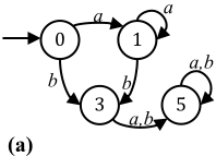
Consider a learner L that actively learns the minimal DQA A that exactly represents the function V : (⌃I )⇤!R from preference information. V maps each input sequence composed from zero or more elements from the input alphabet ⌃I to a real number. Here, A is hQ↪ q0↪⌃I ↪⌃O ↪ δ↪ L↪Vali, with a finite set of states Q, initial state q0 2Q, input and output alphabets ⌃I and ⌃O , transition function δ :Q⇥⌃I !Q, and labeling function L : Q!⌃O which assigns outputs to states. The valuation function Val : (⌃I )⇤!R folds state labels traversed by a sequence into a real value via an aggregation operator ⊕:R⇥R!R. We define the j-length prefix of s as s:j, the length of s as ♣s♣, the concatenation of sequences s (prefix) and e (suffix) as s · e, and an element of ⌃I as σ. The extended transition function ˆ δ :Q⇥(⌃I )⇤ !Q simulates a sequence of transitions with ˆ δ(q0↪ σ · s) = ˆ δ(δ(q0↪ σ)↪ s). Then, A(s)=Val(s)= L♣s♣ j=0L(ˆ δ(q0↪ s:j)) aggregates the traversed state labels. Figure 3a shows a summation example. Q↪ δ, and L are learned from VbP and equivalence queries.

VbP queries yield the relative ordering of two sequences according to V, and equivalence queries indicate whether a hypothesis automaton values every sequence identically to V. We assume the teacher has preferences consistent with V, and responds to preference and equivalence queries as follows:

Definition 1 (Preference Query). A preference query prefQ : (⌃I )⇤ ⇥ (⌃I )⇤ ! ¶1↪ 0↪ -1♦ is evaluated as

Definition 2 (Equivalence Query). An equivalence query returns a triple in B⇥(⌃I )⇤⇥R: is A correct or not; if not, then a counterexample sequence c where the evaluation of c by A and by V do not match; and a real value from feedback function f (c↪ A↪ V) with semantics understood by the learner.

3.1 Preliminaries

Automata learning algorithms learn the states Q, the transition function δ, and the labeling function L for the automaton being learned. Input and output alphabets ⌃I and ⌃O are typically known. An alphabet is a finite set of elements used to construct sequences. A sequence is a list of alphabet elements; an input sequence σ1 · · · σk represents sequence of k transitions taken in an automaton.

L⇤ , Queries, and Observational Equivalence. L⇤ -based learners query a teacher for observations about sequences. Many query types either return the label of a sequence from the output alphabet (e.g. membership queries), or how the labels of a pair of sequences are related (e.g. CbP queries). Observations are recorded in a 2D observation table O. Based on the table structure and the type of observations gathered, an explicit definition for observational equivalence determines if two rows of O represent the same state. States and transitions are identified by applying observational equivalence. Because O is used to represent Q↪ δ, and L of the desired automaton, certain conditions are imposed to ensure O meets the formal automaton definition of the desired automaton. Once this occurs, an automaton can be constructed from O and checked for correctness with an equivalence query to the teacher. Alternation between construction and correctness checks continues until the correct automaton is found. For an in-depth overview of L⇤ , we refer the reader to Appendix B.

Observation Tables and Row Equivalence. An observation table is a 2D array with rows and columns. Each row is indexed by a prefix and each column by a suffix. For a given prefix s and suffix e, the corresponding table entry is the observed label of the sequence s · e. A row indexed by prefix s is denoted row(s). Observational equivalence occurs when two rows are identical: if the observations for each suffix (column) are identical between two rows, those two rows are assumed to represent the same state. Therefore, observational equivalence is defined by row equivalence.

Symbolic Observation Table. By contrast, in a symbolic observation table O, table entries are variables that represent state labels. The variables are related through the constraints C obtained from preference and equivalence queries. Formally, O is the tuple hS↪ E↪ T ; C↪ Γi, where S is the set of prefixes, E is the set of suffixes, C is the set of constraints, context Γ is a bijective mapping from sequences to variables, and the empirical observation function T maps each prefixsuffix sequence s·e 2 (S[(S ·⌃I ))·E indexed in the table to a variable in the context Γ via the mapping T (s · e) = Γ[s · e]. Row equivalence is then defined symbolically.

Symbolic Row Equivalence. Rows row(s1) and row(s2) represent the same state when their entries are the same: for all e 2 E, T(s1 · e) ⌘ T(s2 · e). Determining if two arbitrary table entries are equivalent necessitates equivalence classes of variables and representatives. An equivalence class of variables is a set of variables where all variables are equivalent to each other. The representative of an equivalence class E is an element of E used to represent all of E (App. C.1, Def. 13).

Bijective Construction. Constructing the automaton hQ↪ q0↪ ⌃I ↪ ⌃O ↪ δ↪ L↪Vali is as follows. First, Q is the set of rows of the table. The initial state q0 corresponds to the empty sequence " row:

Transitions between states are computed by appending an element σ from the input alphabet to any prefix s of the current state row(s). Then, the next state is row(s · σ):

Finally, the entries of the " column are used to construct the symbolic labeling ˜L. The labeling function L is resolved by a satisfying solution ⇤ to the constraint set C.

A symbolic hypothesis is a proposed automaton that labels states with ˜L. A concrete hypothesis labels states with L.

Conditions for Construction. The transition function δ for a deterministic automaton has two critical properties. It is deterministic, or consistent, i.e. it is a function. It is also closed, i.e. the range of δ must be a subset of the states in the domain: δ : Q ⇥ ⌃I ! Q0 , where Q0 ✓ Q. Since the table O must represent δ over a finite set of states, O must also exhibit the properties of closedness and consistency prior to constructing a hypothesis automaton from O. Both checks rely on row equivalence.

Unification Enables Row Equivalence. Unification is a two-step process that results in a unified O. First, equivalence classes of variables are determined. Second, O is rewritten in terms of representatives. Unification enables closedness and consistency checks via symbolic row equivalence. Thus, constructing an automaton A using Equations 3-7 requires a unified, closed, and consistent table O.

Equivalence Queries and Counterexample Processing. The learner always requests a check of the constructed A via an equivalence query. If A is correct, the learner terminates. If A is incorrect, a counterexample c is received from the teacher and incorporated into the table by the learner. L⇤ specifically adds c and all prefixes of c to S. Alternatives exist, such as adding c and all suffixes of c to E. The purpose of expanding the table with c is to correct Q, δ, or L.

Formal Theories. A theory is a set of axioms and all statements which can be logically derived from those axioms.

4 QUINTIC

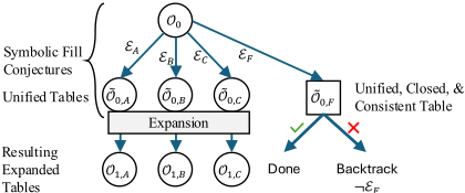
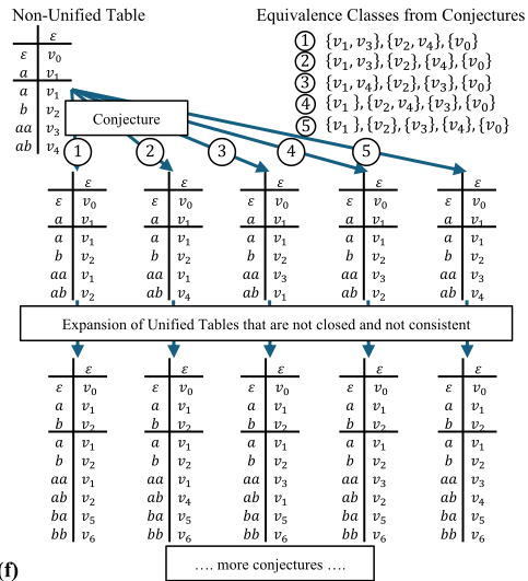
To learn minimal DQAs, QUINTIC (Figure 1; Algorithm 1) deductively reasons within the theory of reals about equivalence classes of variables. A class E is valid if it satisfies the current constraints C gathered in the symbolic observation table O. Choosing a satisfying E allows QUINTIC to unify O into a unified table ˜O. However, in order to hypothesize a set of states Q, transition function δ, and symbolic labeling ˜L, the unified table ˜Omust be closed and consistent. If ˜O fails to be closed and consistent, then the table must be expanded and an additional E must be chosen. Because C may permit multiple satisfying solutions for E that remain unverifiable until an equivalence query is executed, each choice of E is considered a conjecture. The process of alternating between choosing an E and expanding O generates a conjecture-expansion chain (CE chain). Hence, identifying the minimal DQA is an uninformed search over CE chains that terminates once an O is found corresponding to the minimal DQA.

Conjecture-Expansion Chains

CE chains are produced by alternating between SYMBOLICFILL (Equation 8) and TABLEEXPANSION (Equation 9) as shown in Figure 1 and lines 3-6 and 20-24 of Algorithm 1:

h(Ek↪Ok)i0kd denotes a (d+1)-length CE chain. Only when Od = ˜Od can a hypothesis automaton be constructed, verified, and an incorrect conjecture be detected. Figure 2 illustrates a tree of possible chains, and Figure 3f illustrates the first few tables of each chain based on the applied conjecture.

Incorrect conjectures are handled through iterative deepening depth first search (IDS) and backtracking. By budgeting the number of times unification occurs, IDS avoids infinite length CE chains. Backtracking undoes table expansions from incorrect conjectures: if the conjunction of constraints, counterexample feedback, and conjectures is unsatisfiable, then the most recent conjecture E is negated under context Γ with at most m variables via logical implication, as shown on the backtracking arrow in Figure 1 and lines 12-13 of Algorithm 1:

If all E have been ruled out under m variables, the table O must be expanded to include more than m variables.

From Queries to Variable Equivalence Conjectures

To gather constraints and determine the set of conjectures to choose E from, preference and equivalence queries are asked and responses are formalized by semantics into Valconstraints (constraints written in terms of the function Val).

Definition 3 (Preference Query Semantics). prefQ returns an element from ¶1↪ 0↪-1♦, corresponding to the relation R2¶>↪ =↪ <♦ in the statement V(s1) RV(s2). The statement is interpreted as V(s1)RV(s2) =)Val(s1)RVal(s2).

Definition 4 (Feedback Semantics). equivQ returns a feedback value f(c↪A↪ V). The strength of feedback provided indicates how the feedback is interpreted. If f is strong, then

meaning the concrete valuation of c is V(c). If f is weak, then

A recursive definition of Val enables Val-constraints to be converted into T-constraints (constraints written in terms of table variables). We consider four valuation functions with recursive formulations: summation (⌃), discounted summation (γ⌃), product (⇧), and classification (N) (definitions in App. C.2). The recursive form for ⌃ is Val(s·σ) = T (s·σ) + Val(s) with Val(") = T (") = 0. Figure 3b shows conversion from Val-constraints to Tconstraints in terms of table variables v0↪ v1↪ and v2 with ⌃. Val leaves variables unbound; A binds variables to values.

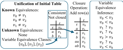
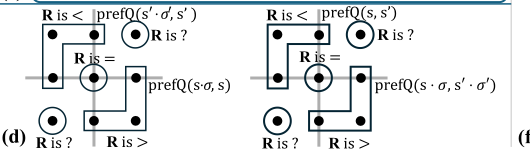
Furthermore, the statement between a pair of table variables T (s·σ)RT (s0 ·σ0 ) can be rewritten in terms of Val (Figure 3c). Specific combinations of preference queries encoded in the Figure 3d decision tree enable the relation R to be inferred. Variable pairs for which R is unique are considered known equivalences, while variable pairs for which R is not unique are considered unknown or ambiguous equivalences.

Selecting a E requires each ambiguous R to be individually assigned either an equality (=) or inequality (6=). A MaxSMT

¬ℰ𝐹

Figure 2: Diagram of Conjecture Expansion Chains. O0 is nonunified. ˜O0↪K is unified after applying conjecture EK. O1↪K is the expansion step if the unified table is not closed or not consistent.

% & = 0

% ( = 0+1 = 1

% * = 0+3 = 3

% (( = 0+1+1 = 2

% (* = 0+1+3 = 4

% *( = 0+3+5 = 8

% ** = 0+3+5 = 8

% ((( = 3

% ((* = 5

% (*( = 9

% (** = 9

% *(( = 13

Initial Symbolic Observation Table ⟨2, 4, 5; 7, Γ⟩ Entries

Constraints 7 from Preference Queries

(c)

(e)

Updated Known Equivalences:

T" ≠ T#

T" ≠ T$

T# ≠ T$

T" ≠ T%

T" ≠ T&

T$ ≠ T%

T% ≠ T&

Updated Unknown Equivalences:

T# ? T%

T# ? T&

T$ ? T&

To proceed with unification, must conjecture variable equivalences for unknown variable equivalences

MaxSMT objective provides an order for trying conjectures:

Maximize number of equalities in (T#?T%) ∧ T#?T& ∧ (T$?T&) subject to the known variable equivalences.

(T#= T%) ∧ T# = T& ∧ T$ = T& UNSAT due to (T#≠ T$)

(T#= T%) ∧ T# ≠ T& ∧ (T$ = T&) SAT

(T#≠ T%) ∧ T# = T& ∧ (T$ = T&) UNSAT due to (T#≠ T$)

(T#= T%) ∧ T# ≠ T& ∧ (T$ ≠ T&) SAT

(T#≠ T%) ∧ T# = T& ∧ (T$ ≠ T&) SAT

(T#≠ T%) ∧ T# ≠ T& ∧ (T$ = T&) SAT

(T#≠ T%) ∧ T# ≠ T& ∧ (T$ ≠ T&) SAT

2

4

1

3

5

Recursive Valuation: 123 4 ⋅ 6 = 8 4 ⋅ 6 +123 4 , Val ; = 8(;) Inference Goal: 8 4 ⋅ 6 A 8 4 ! ⋅ 6! identify relation A ∈ {=,<,>} Rewrite recursive form: 8 4 ⋅ 6 = 123(4 ⋅ 6) -123(4) Rewritten Goal: 123(4 ⋅ 6) -123(4) A 123(4′ ⋅ 6′) -123(4′) Equivalent Variable Inference Goal after Rearrangement: 8 4 ⋅ 6 A 8 4 ! ⋅ 6! ⟺Val 4 ⋅ 6 +Val 4 ! A Val 4 ! ⋅ 6! +Val 4

Variable Inference, given constraints from Preference Queries

Desired Relation

Inference Goal

Equivalent Goal

Algorithm 1 QUINTIC Algorithm

1: Init k=0, Ok =hS↪E↪ T; C↪ Γi, S = E = ¶"♦, C = ¶♦, Γ = ;, and cexes = ¶♦, correct? = False 2: ˜Ok↪ Ck↪ Ek = SYMBOLICFILL(Ok) 3: while not ISCLOSEDANDCONSISTENT( ˜Ok) do 4: Ok+1 = EXPANDIFNOTCLOSEDCONSISTENT( ˜Ok) 5: ˜Ok+1↪ Ck+1↪ Ek+1 = SYMBOLICFILL(Ok+1); k++ 6: end while 7: HS = MAKESYMBOLICHYPOTHESIS( ˜Ok↪⌃I ↪⌃O ) 8: while not correct? do 9: ⇤k↪ sat? = SOLVE(Ck↪ Ek↪HS↪ cexes) 10: if sat? is UNSAT then 11: Ok-1 = PROCESSCEX(Ok-1↪ cexes) 12: Ck-1 = Ck ^ (g  ♣Γ♣ =) ≻Ek) 13: k k -1, and then goto Line 2 14: end if 15: h = MAKECONCRETEHYPOTHESIS(HS↪⇤k) 16: correct?, cex, feedback = EQUIVALENCEQUERY(h) 17: cexes.ADD((cex, feedback)) 18: end while 19: return h 20: procedure SYMBOLICFILL(Ok) 21: Ck = GETCONSTRAINTSVIAPREFQUERIES(Ok) 22: Ek = CONJECTUREORDERBYMAXSMT(Ok↪ Ck) 23: ˜Ok = UNIFICATION(Ek↪ Ok) 24: return ˜Ok↪ Ck↪ Ek 25: end procedure

objective over the set of ambiguous relations prioritizes the order in which conjectures are chosen. Maximizing the number of variable equalities is a rough proxy for minimizing the number of states in the automaton. Figure 3e illustrates how an ordering over conjectures is produced by the MaxSMT objective. Other MaxSMT objectives, such as prioritizing closed and consistent tables, can also be utilized. Unification proceeds once all ambiguous R have been conjectured.

Counterexample Processing

Counterexample processing is identical to L⇤ , informatively directs table expansion, and yet is unnecessary for complete search due to Equation 10 which detects required expansions. Appendix E.7 analyzes impact of counterexample processing.

5 Theoretical Guarantees of QUINTIC

Our analysis of QUINTIC considers minimalism and completeness guarantees, followed by analysis of query complexity of the algorithm. Full proofs are deferred to Appendix D.

Theorem1 (MinimalismandCompleteness). If n is the number of states of the minimal automaton isomorphic to the target, then QUINTIC correctly terminates after finite expansion operations with an n state automaton at the end of a CE chain containing at most n - 1 expansion operations.

Proof Sketch. Minimalism and completeness are a consequence of (1) the completeness of IDS, whether in a constrained or unconstrained solution space, (2) showing a bijection between partitions of conjectures and the number of states in the table, and (3) showing the correct solution must exist on a CE chain of at most length n - 1.

Theorem 2 (Query Complexity). If n is the number of states of the minimal automaton isomorphic to the target, and m is the maximum length of any counterexample the teacher returns, then (a) QUINTIC executes at most N= n2 ♣⌃O ♣n{♣⌃I ♣n n equivalence queries, where {rt is a Stirling number of the second kind (the number of ways to partition r elements into t non-empty subsets), and (b) the preference query complexity is at most O (♣⌃I ♣(n + mN)3 log(♣⌃I ♣(n + mN)3 )).

Proof Sketch. The number of equivalence queries leverages results from Theorem 1 and Bassino and Nicaud to upper bound the number of automata Ak with k states [Bassino and Nicaud, 2007]; a bound for the sum of Ak over k from 1 to n yields the equivalence query result. Preference query complexity depends on ♣(S [ (S · ⌃I )) · E♣, which is upper bounded by table size ♣E♣♣S♣(1 + ♣⌃I ♣). To obtain the preference query complexity result, analyze the maximum size of the table based on a budget of n-1 expansion operations.

6 Empirical Results

Our evaluations show how (1) query complexity and (2) solver time scale as a function of feedback strength, MaxSMT objective, and valuation function. The query complexity of QUINTIC is generally larger than REMAP, but surprisingly, QUINTIC achieves better query complexity than REMAP under classification-based preferences (CbPs).

6.1 Experimental Setup

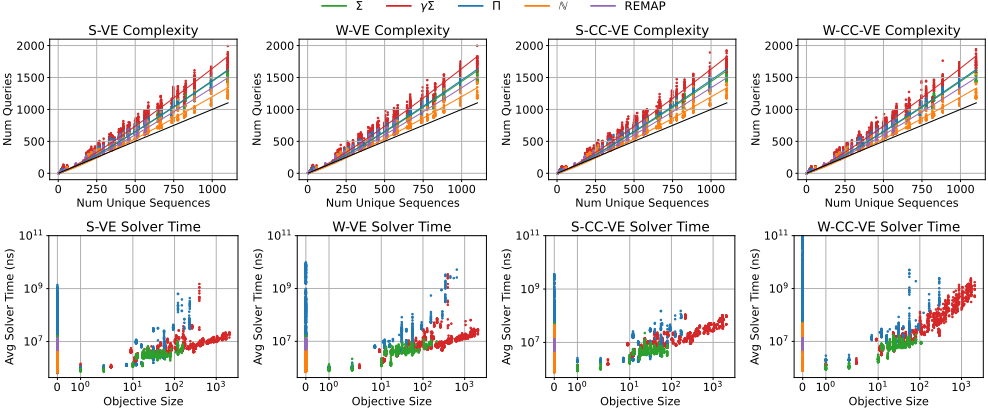
We compare QUINTIC to REMAP, a CbP learning method with strong feedback and no backtracking. Query complexity and solver time were measured for learning 25 automata. We varied feedback strength and MaxSMT objectives for QUINTIC. Each automaton (shown in Appendix E.2) has four versions, one for each valuation function investigated. Results are shown in Figure 4.

Valuation Functions, Output Alphabet, and Theories. The Val function and ⌃O correspond to a minimal theory QUINTIC reasons over. Theory of rationals (TQ) applies to: (1) both ⌃ and γ⌃ with a rational ⌃O and (2) ⇧ with a positive rational ⌃O . Theory of total ordering applies to N with a finite ⌃O of classes represented by integers.

QUINTIC Variants. We evaluate 4 variants of QUINTIC based on choice of feedback and MaxSMT objective. Feedback is strong (S) (Equation 11) or weak (W) (Equation 12). For MaxSMT objectives, we maximize the number of variable equalities (VE) (Appendix C.6 Equation 29 defines the VE objective). Alternatively, we maximize VE in conjunction with an objective simulating a 1-step lookahead for closedness and consistency (CC-VE) (Appendix C.7 details the CC objective). Therefore, the four variants are strong-variable-equality (S-VE), weak-variable-equality (WVE), strong-closed-consistent-variable-equality (S-CC-VE), and weak-closed-consistent-variable-equality (W-CC-VE).

Baseline. REMAP can only handle CbP queries. Variants S-VE and S-CC-VE under CbP are most similar to REMAP.

Implementation. Each QUINTIC variation is run 100 times per automaton, for a total of 2500 trials per variant, and 10000 trials overall. Counts of preference and equivalence queries and total solver time are measured per trial. Constraints are encoded using a rational representation; Z3 is used for SMT and MaxSMT solving [De Moura and Bjørner, 2008]. Exact equivalence queries are implemented with the Hopcroft-Karp algorithm which checks for equivalence by inspecting the transition function and state labels [Hopcroft and Karp, 1971; Almeida et al., 2009]. Such a check is equivalent to computing the valuations for infinitely many sequences.

6.2 Scaling Results

We measure scaling in two ways. First, we plot preference query complexity as a function of the number of unique sequences in the table. Second, we plot mean solver time versus MaxSMT objective size in order to determine how expensive finding satisfying solutions is under γ⌃↪⌃↪⇧, and N.

Query Complexity. The preference query complexity of each QUINTIC variant under the γ⌃↪⌃↪⇧, and N valuationbased preference queries are shown in the top row of Figure 4. In order of decreasing preference query complexity, the bestfit curves are γ⌃, ⇧, ⌃, REMAP, and N, with a small difference between ⇧ and ⌃. The order of curves for REMAP and N appears to contradict the notion that REMAP represents a lower bound on preference query complexity. However, the maximum number of unique sequences for REMAP is roughly half the maximum of the other valuations, implying that QUINTIC requires larger tables and more queries than REMAP. Suffix set E does not need to be prefix-closed for REMAP, but QUINTIC requires E to be prefix-closed. Therefore, QUINTIC ends up with larger tables than REMAP.

Solver Time. Mean solver time is compared to MaxSMT objective size in the bottom row of Figure 4. QUINTIC solves large numbers of unknown variable relations, as measured by MaxSMT objectives involving at least 1000 terms. Learning under γ⌃ generates large MaxSMT objectives for some automata. Although CE chain length typically does not surpass 50 when learning the 25 automata, the total solver time can be quite expensive for certain targets, especially under ⇧, weak feedback, and the CC-VE objective. In fact, the solving time depends on the valuation function used and theories employed in Z3. Solving under ⇧ is the most expensive, while γ⌃ generates large objectives that are still relatively quick to solve. Additional results in Appendix Figure 14 indicate QUINTIC tends to gather significantly more inequalities than REMAP. Solving time for nonlinear inequalities is expensive, as evidenced by ⇧. However, large numbers of linear inequalities, from γ⌃, are efficiently solvable.

7 Limitations and Conclusion

QUINTIC is an L⇤ -based algorithm for actively learning deterministic quantitative automata from constraints obtained from preference queries and feedback. We consider how QUINTIC learns under summation, discounted summation, product, and classification valuation functions. Significantly improving query complexity of QUINTIC would allow for use cases where humans can be queried directly for preferences. Dropping exactness in favor of probably approximately correct identification would enable a tradeoff between budgeting sampling-based equivalence queries and solution error tolerance. Conjectured variable equivalences, guided by a MaxSMT objective and iterative deepening search, ensures search completeness and minimalism in QUINTIC. We investigate how QUINTIC scales under different valuation functions, feedback strength, and MaxSMT objective.

Acknowledgements

This work has taken place in the Autonomous Mobile Robotics Laboratory (AMRL) and the Trishul Lab in the University of Texas at Austin Computer Science Artificial Intelligence Lab. AMRL research is supported in part by the NSF (CAREER-2046955, IIS-2416461, CCF2505865, DGE-2125858). Trishul research is supported in part by DARPA (HR00112320018, HR0011-24-9-0431) and the Army Research Office (W911NF2110009). The views and conclusions contained in this document are those of the authors alone.