
Transforming and Encoding FTS for SAT Solving: What Helps, What Hurts
Proceedings of the Thirty-Fifth International Joint Conference on Artificial Intelligence. Main Track. Pages 2236-2246.
https://doi.org/10.24963/ijcai.2026/249
© 2026 International Joint Conferences on Artificial Intelligence
Keywords
- Constraint Satisfaction and Optimization: Satisfiabilty
- Planning and Scheduling: Activity and plan recognition
Abstract
Factored tasks are a classical planning representation that extends SAS+ with limited forms of disjunctive preconditions, conditional effects, and angelic nondeterminism. This added expressiveness allows for a more compact representation of taks than traditional formalisms such as STRIPS or SAS+, and supports a wide range of task transformations. However, existing planning approaches for factored tasks have been limited to heuristic search methods.
In this work, we investigate how to encode factored tasks in SAT. We propose several ways to encode the tasks, focusing on different strategies for translating the factored transition relation into propositional logic. We also analyze how to exploit parallelism at various levels in this setting and study the impact of common task transformations on the performance of SAT-based planners.
- [Bäckström and Nebel, 1995] Christer Bäckström and Bern- hard Nebel. Complexity results for SAS + planning. Com- putational Intelligence, 11(4):625-655, 1995.
- [Behnke et al., 2025] Gregor Behnke, David Speck, and Daniel Gnad. Axsat-bringing axioms to sat planning. In European Conference on Logics in Artificial Intelligence, pages 77-93. Springer, 2025.
- [Bernardini and Muise, 2024] Sara Bernardini and Christian Muise, editors. Proceedings of the Thirty-Fourth Interna- tional Conference on Automated Planning and Scheduling (ICAPS 2024). AAAI Press, 2024.
- [Biere et al., 2024] Armin Biere, Tobias Faller, Katalin Fazekas, Mathias Fleury, Nils Froleyks, and Florian Pol- litt. CaDiCaL, Gimsatul, IsaSAT and Kissat entering the SAT Competition 2024. In Marijn Heule, Markus Iser, Matti Järvisalo, and Martin Suda, editors, Proc. of SAT Competition 2024 -Solver, Benchmark and Proof Checker Descriptions, volume B-2024-1 of Department of Com- puter Science Report Series B, pages 8-10. University of Helsinki, 2024.
- [Büchner et al., 2024] Clemens Büchner, Patrick Ferber, Jendrik Seipp, and Malte Helmert. Abstraction heuristics for factored tasks. In Bernardini and Muise [2024], pages 40-49.
- [Domshlak et al., 2009] Carmel Domshlak, Jörg Hoffmann, and Ashish Sabharwal. Friends or foes? On planning as satisfiability and abstract CNF encodings. Journal of Arti- ficial Intelligence Research, 36:415-469, 2009.
- [Fan et al., 2014] Gaojian Fan, Martin Müller, and Robert Holte. Non-linear merging strategies for merge-and-shrink based on variable interactions. In Stefan Edelkamp and Roman Barták, editors, Proceedings of the Seventh Annual Symposium on Combinatorial Search (SoCS 2014), pages 53-61. AAAI Press, 2014.
- [Fikes and Nilsson, 1971] Richard E. Fikes and Nils J. Nils- son. STRIPS: A new approach to the application of the- orem proving to problem solving. Artificial Intelligence, 2:189-208, 1971. IJCAI
- [Filipe et al., 2026a] João Filipe, Álvaro Torralba, and Gre- gor Behnke. (data and code) transforming and encod- ing fts for sat solving: What helps, what hurts. https: //doi.org/10.5281/zenodo.20444380, 2026. DOI
- [Filipe et al., 2026b] João Filipe, Álvaro Torralba, and Gre- gor Behnke. (extended version) transforming and encod- ing fts for sat solving: What helps, what hurts. https: //arxiv.org/abs/, 2026. Link
- [Froleyks et al., 2019] Nils Christian Froleyks, Tomás Ba- lyo, and Dominik Schreiber. PASAR -planning as sat- isfiability with abstraction refinement. In Pavel Surynek and William Yeoh, editors, Proceedings of the 12th An- nual Symposium on Combinatorial Search (SoCS 2019), pages 70-78. AAAI Press, 2019.
- [Helmert et al., 2014] Malte Helmert, Patrik Haslum, Jörg Hoffmann, and Raz Nissim. Merge-and-shrink abstrac- tion: A method for generating lower bounds in factored state spaces. Journal of the ACM, 61(3):16:1-63, 2014.
- [Helmert, 2006] Malte Helmert. The Fast Downward plan- ning system. Journal of Artificial Intelligence Research, 26:191-246, 2006.
- [Hoffmann and Nebel, 2001] Jörg Hoffmann and Bernhard Nebel. The FF planning system: Fast plan generation through heuristic search. Journal of Artificial Intelligence Research, 14:253-302, 2001.
- [Hoffmann et al., 2014] Jörg Hoffmann, Peter Kissmann, and Álvaro Torralba. "Distance"? Who cares? Tailor- ing merge-and-shrink heuristics to detect unsolvability. In Torsten Schaub, Gerhard Friedrich, and Barry O'Sullivan, editors, Proceedings of the 21st European Conference on Artificial Intelligence (ECAI 2014), pages 441-446. IOS Press, 2014.
- [Huang et al., 2012] Ruoyun Huang, Yixin Chen, and Weix- iong Zhang. SAS + planning as satisfiability. Journal of Artificial Intelligence Research, 43:293-328, 2012.
- [Kautz and Selman, 1992] Henry Kautz and Bart Selman. Planning as satisfiability. In Bernd Neumann, editor, Pro- ceedings of the 10th European Conference on Artificial In- telligence (ECAI 1992), pages 359-363.
- [Kautz and Selman, 1996] Henry Kautz and Bart Selman. Pushing the envelope: Planning, propositional logic, and stochastic search. In Proceedings of the Thirteenth Na- tional Conference on Artificial Intelligence (AAAI 1996), pages 1194-1201. AAAI Press, 1996.
- [Kautz et al., 2006] Henry Kautz, Bart Selman, and Jörg Hoffmann. SatPlan: Planning as satisfiability. In Fifth International Planning Competition (IPC-5): Planner Ab- stracts, 2006.
- [Korf, 1997] Richard E. Korf. Finding optimal solutions to Rubik's Cube using pattern databases. In Proceedings of the Fourteenth National Conference on Artificial Intelli- gence (AAAI 1997), pages 700-705. AAAI Press, 1997.
- [Nebel, 2000] Bernhard Nebel. On the compilability and expressive power of propositional planning formalisms. Journal of Artificial Intelligence Research, 12:271-315, 2000.
- [Rintanen et al., 2006] Jussi Rintanen, Keijo Heljanko, and Ilkka Niemelä. Planning as satisfiability: parallel plans and algorithms for plan search. Artificial Intelligence, 170(12-13):1031-1080, 2006.
- [Rintanen, 2011] Jussi Rintanen. Madagascar: Scalable planning with SAT. In IPC 2011 Planner Abstracts, pages 61-64, 2011.
- [Rintanen, 2012] Jussi Rintanen. Planning as satisfiability: Heuristics. Artificial Intelligence, 193:45-86, 2012.
- [Rintanen, 2014] Jussi Rintanen. Madagascar: Scalable planning with SAT. In Eighth International Planning Competition (IPC-8): Planner Abstracts, pages 66-70, 2014.
- [Robinson et al., 2009] Nathan Robinson, Charles Gretton, Duc Nghia Pham, and Abdul Sattar. SAT-based parallel planning using a split representation of actions. In Al- fonso Gerevini, Adele Howe, Amedeo Cesta, and Ioannis Refanidis, editors, Proceedings of the Nineteenth Interna- tional Conference on Automated Planning and Scheduling (ICAPS 2009), pages 281-288. AAAI Press, 2009.
- [Seipp et al., 2017] Jendrik Seipp, Florian Pommerening, Silvan Sievers, and Malte Helmert. Downward Lab. https: //doi.org/10.5281/zenodo.790461, 2017. DOI
- [Sievers and Helmert, 2021] Silvan Sievers and Malte Helmert. Merge-and-shrink: A compositional theory of transformations of factored transition systems. Journal of Artificial Intelligence Research, 71:781-883, 2021.
- [Sievers et al., 2014] Silvan Sievers, Martin Wehrle, and Malte Helmert. Generalized label reduction for merge- and-shrink heuristics. In Carla E. Brodley and Peter Stone, editors, Proceedings of the Twenty-Eighth AAAI Confer- ence on Artificial Intelligence (AAAI 2014), pages 2358- 2366. AAAI Press, 2014.
- [Sievers et al., 2016] Silvan Sievers, Martin Wehrle, and Malte Helmert. An analysis of merge strategies for merge-and-shrink heuristics. In Amanda Coles, Andrew Coles, Stefan Edelkamp, Daniele Magazzeni, and Scott Sanner, editors, Proceedings of the Twenty-Sixth Interna- tional Conference on Automated Planning and Scheduling (ICAPS 2016), pages 294-298. AAAI Press, 2016.
- [Sievers et al., 2024] Silvan Sievers, Thomas Keller, and Gabriele Röger. Merging or computing saturated cost partitionings? a merge strategy for the merge-and-shrink framework. In Bernardini and Muise [2024], pages 541- 545.
- [Sievers, 2018] Silvan Sievers. Merge-and-shrink heuristics for classical planning: Efficient implementation and par- tial abstractions. In Vadim Bulitko and Sabine Storandt, editors, Proceedings of the 11th Annual Symposium on Combinatorial Search (SoCS 2018), pages 90-98. AAAI Press, 2018.
- [Sinz, 2005] Carsten Sinz. Towards an optimal CNF encod- ing of boolean cardinality constrai nts. In Proceedings of the 11th International Conference on Principles and Prac- tice of Constraint Programming (CP 2005), volume 3709, pages 827-831. Springer, 2005.
- [Speck et al., 2023] David Speck, Paul Höft, Daniel Gnad, and Jendrik Seipp. Finding matrix multiplication al- gorithms with classical planning. In Sven Koenig, Roni Stern, and Mauro Vallati, editors, Proceedings of the Thirty-Third International Conference on Automated Planning and Scheduling (ICAPS 2023), pages 411-416. AAAI Press, 2023.
- [Torralba and Sievers, 2019] Álvaro Torralba and Silvan Sievers. Merge-and-shrink task reformulation for classi- cal planning. In Sarit Kraus, editor, Proceedings of the 28th International Joint Conference on Artificial Intelli- gence (IJCAI 2019), pages 5644-5652. IJCAI, 2019. IJCAI
- [Torralba et al., 2017] Álvaro Torralba, Vidal Alcázar, Pe- ter Kissmann, and Stefan Edelkamp. Efficient symbolic search for cost-optimal planning. Artificial Intelligence, 242:52-79, 2017.
- [Torralba et al., 2023] Álvaro Torralba, Silvan Sievers, Ras- mus G. Tollund, and Kristian Ø. Nielsen. FTSPlan: Task reformulation via merge-and-shrink. In Tenth Interna- tional Planning Competition (IPC-10): Planner Abstracts, 2023.
References were extracted automatically from the PDF and may contain errors.
Full text extracted automatically from the PDF; figures, tables and equations may differ. The PDF is the version of record.
1 Introduction
Classical planning algorithms aim to exploit a model of the environment to find a plan. Different representations can be used to model the environment, e.g., STRIPS [Fikes and Nilsson, 1971] or SAS+ [B¨ackstr¨om and Nebel, 1995], offering a trade-off between expressiveness and ease to exploit for planning algorithms. We consider planning tasks in a factored transition system (FTS) representation, where states are described in terms of finite-domain variables, and each variable (also called factor) is described as a transition system. This provides a lot of flexibility for expressing the possible behaviors (preconditions and effects) of an action within one variable, provided independence of this behavior across variables. The FTS representation was originally considered in the context of merge-and-shrink abstractions [Helmert et al., 2014], but was later adopted as a planning task representation due to having several advantages over previous representations. Compared to SAS+, for example, we can easily express for each variable disjunctive preconditions, conditional effects, and even angelic non-determinism (where we can choose multiple outcomes for a given action). Expressing the same transition semantics in SAS+ requires either exponential-size compilation or introducing auxiliary state variables and operators that increase plan length [Nebel,
2000; B¨uchner et al., 2024]. On the one hand, it allows to naturally encode domains that are not easy to express in SAS+, such as finding algorithms for matrix multiplication [Speck et al., 2023], or Rubik's cube [Korf, 1997; B¨uchner et al., 2024]. On the other hand, it provides a very flexible representation for task transformation [Torralba and Sievers, 2019; Sievers and Helmert, 2021].
Thus, it is desirable to have planning methods that support this representation natively. So far, existing planning approaches for factored tasks have focused more on optimal planning, using heuristic search methods with admissible heuristics [Torralba and Sievers, 2019; B¨uchner et al., 2024], or symbolic search [Torralba et al., 2017; Torralba et al., 2023]. For agile planning, only heuristic search algorithms exist [Torralba and Sievers, 2019; Torralba et al., 2023]. These are not always suitable for the FTS representation. For example, an FTS can encode tasks with exponential branching factor in the size of the task, where straightforward heuristic search approaches fail immediately.
SAT-based planning has been a prominent approach since the early work of Kautz and Selman [1992]. The general idea is to encode the existence of a plan of length N as a propositional formula ϕN, which is satisfiable if and only if such a plan exists. This formula is then passed to a SAT solver, either incrementally increasing N for optimal planning, or following a schedule for satisficing planning [Rintanen, 2012; Rintanen, 2011]. Over the years, several SATbased planning systems have been developed, such as SATPLAN04 [Kautz et al., 2006], Madagascar [Rintanen, 2012], action splitting [Robinson et al., 2009], abstract CNF encodings [Domshlak et al., 2009] PASAR [Froleyks et al., 2019], AxSAT [Behnke et al., 2025], and SASE [Huang et al., 2012], each contributing different encoding strategies or solver techniques. However, these systems typically target classical representations and are not directly applicable to FTS tasks. Adapting SAT planning to this setting enables new encoding strategies that make better use of the structure inherent in factored models.
In this work, we consider several alternative ways to encode FTS planning tasks as a SAT formula. While a naive encoding is straightforward, we propose several encodings for the transition relation, as well as exploiting parallelism. Our experiments show that these optimizations are fundamental to achieve a good performance, that SAT-based planning can be competitive as well for solving factored tasks, and have good synergy with task reformulation methods.
2 Preliminaries
A transition system (TS) is a tuple Θ = ⟨S,L, T, sI , SG⟩ where S is a finite set of states, L is a finite set of labels, T ⊆ S×L×S is a set of transitions, sI ∈ S is the initial state, and SG ⊆ S is the set of goal states. A path s l1 -→ . . . lk -→ t from s to t is a sequence of k transitions (si-1, li, si) ∈ T for 1 ≤ i ≤ k, starting in s = s0 and ending in t = sk. A plan for s is a path from s to any s′ ∈ SG.
2.1 Factored Tasks
We consider planning tasks in a factored transition system representation, where states are described in terms of finitedomain variables, and each variable (also called factor) is described as a TS [Helmert et al., 2014; Torralba and Sievers, 2019; Sievers and Helmert, 2021; B¨uchner et al., 2024]. A factored task T = ⟨Θ1, . . . , Θn⟩ is a tuple of TSs with a common set of labels, L, such that Θi = ⟨Si,L, Ti, sIi , SG i ⟩ for 1 ≤ i ≤ n. We assume that all Si are disjoint, i.e., Si ∩ Sj = ∅. We characterize the size of task T in terms of the number of factors |T | = n, the number of labels |L|, and the maximum number of states in each factor D = maxΘi∈T |Si|.
This is a compact representation of a state space, which is the synchronized product Θ⊗ = ⊗ni=1 Θi of all factors. A state in Θ⊗ is a tuple of states from the individual factors s = ⟨s1, . . . , sn⟩, one for each factor, si ∈ Si. The state space of a factored task is the synchronized product of all its factors. This is another transition system ΘT = Θi ⊗ . . . ⊗ Θn = ⟨ST , L, TT , sIT , SG T ⟩, where ST = S1 × · · ·×Sn is the Cartesian product of each factor's states, TT = {(⟨s1, . . . , sn⟩, l, ⟨t1, . . . , tn⟩) | (si, l, ti) ∈ Ti for 1 ≤ i ≤ n}, sIT = ⟨sI1 , . . . , sIn ⟩, and SG T = SG 1 × · · · ×SG n .
2.2 Task Transformation
Apart from being able to easily express some planning tasks more naturally than other formalisms, an advantage of using the factored representation is that a large number of transformations are available [Sievers and Helmert, 2021]. Though many of these transformations are tailored towards creating abstractions of the task, some of them can also be used to simplify the task before solving it, if they have the property that a plan for the original task can be reconstructed from any plan for the transformed task [Torralba and Sievers, 2019]. Some of the transformations available include:
- Label reduction [Sievers et al., 2014] reduces the set of labels while keeping the set of transitions of the product TS intact (up to label renaming).
- Weak-bisimulation shrinking [Hoffmann et al., 2014] reduces the number of states in a factor. This may change the goal distance of states in Θ⊗, but it preserves whether states were solvable or not so that a solution for the original task can be reconstructed.
- Pruning unreachable and dead-end states in the factors [Sievers and Helmert, 2021].
- Merging two or more factors into one [Fan et al., 2014; Sievers et al., 2016; Sievers et al., 2024]. This reduces the number of factors, at the cost of increasing their size exponentially in the number of combined factors.
These transformations can be combined, having synergies [Sievers and Helmert, 2021]. For example, pruning typically is not applicable on the input task, but merging factors may lead to discovering that many of the combined states are unreachable or dead-ends. Notably, the transformations make use of the expressiveness of the representation. A factored task obtained from compiling a SAS+ task will never have non-deterministic labels or disjunctive preconditions. However, label reduction or shrinking may introduce them.
2.3 Boolean Satisfiability
Boolean Satisfiability (SAT) is the task of determining whether a propositional formula in conjunctive normal form (CNF) has a truth assignment of its variables that makes the formula true. A CNF formula consists of a conjunction (∧) of clauses, where each clause is a disjunction (∨) of literals. A literal is a propositional variable, or variable for short, x or its negation ¬x. SAT solvers, which are readily available, determine whether a formula is satisfiable, and if so, provide a satisfying truth assignment. For ease of notation, we will not present the SAT formulae in this paper in CNF, but all formulae can be translated easily to CNF.
3 SAT Planning
The general idea in SAT planning is to, given a planning task and a bound on the number of timesteps N, construct a SAT formula that is satisfiable if and only if there exists a plan with a makespan of N. Our encodings use the following variables, for each timestep t ∈ {0, . . . , N}:
- sti : indicates if we are at state si ∈ Θk at timestep t.
- lt : indicates if a label l ∈ L is selected at timestep t.
Then, we need to encode constraints that ensure that the values of these variables correspond to an executable and goal-reaching path. In each factor, we have to be exactly in one state at every timestep. To enforce this, we assert that at least one state in each factor has to be selected via a disjunction (∨) across all states of that factor. We also assert that at most one state in the factor is selected. Depending on the number of variables, its encoding varies. For up to 256 variables, a naive quadratic encoding is used, whereas a binary counter encoding is applied otherwise [Sinz, 2005].
Additionally, the initial and goal states are enforced at the first and last timesteps respectively.
Finally, we must ensure that consecutive layers are consistent with the transition relation, i.e., for each t, st+1 can be reached from st by applying the selected labels lt . Next, we focus on encoding the transition relation under the restriction that a single label can be selected at each timestamp.
We will relax these constraints when we discuss parallelism.
4 Encoding of the Transition Relation
We present several ways to encode FTS tasks into SAT, which leverage the structure of the FTS representation. In an FTS task, labels capture all the dependencies across factors. So, it suffices to encode each Θk separately, restricting which pairs of states sti , st+1 j ∈ Sk are consistent with the label lt selected at time t. We describe the encoding for a single factor Θk and timestep t. The final SAT formula is the conjunction of the encoding for every factor and time step, in addition to constraints 1 to 6.
The transition relation Tk can be seen as a 3D structure (with dimensions: source, target and label) indicating whether a transition is valid for a given triple of values. In a SAT encoding, the constraints do not "build solutions" directly but rule out those assignments that do not correspond to possible transitions. The simplest encoding of Tk is to explicitly list every impossible transition. Since at every timestep a state and a label must be chosen (constraints 1, 2, 5 and 6), the chosen transition must be one allowed in Tk. We call these constraints forbidding transitions primal constraints.
Together constraints (1) through (7) already constitute a complete encoding of the FTS task as a SAT formula - which will be our baseline encoding. This encoding can be quite inefficient in terms of the number of clauses, as constraint 7 requires O(|L| · |T | ·D2 ) clauses. It is also fairly inflexible as it only asserts that transitions that are not present in the transition system cannot be used and does not leverage in any way the information of valid transitions. In the rest of the section we develop alternative ways of encoding equivalent formulas with the same satisfying assignments.
4.1 Constraint-per-line Encoding
Constraint 7 excludes transitions that do not exist in Tk. Each such constraint can be written as an implication stating that if two of the values are selected, then the third one cannot be selected: e.g. if we focus on the target state: lt ∧ sti =⇒ ¬st+1 j . We can now aggregate all such implications for label l and source state si into a single formula.
When focusing on a single label l, the transitions for l in Tk describe an adjacency matrix between the source and target states. Constraint 8 then encodes each row of l's adjacency matrix by forbidding targets which cannot be reached from the source corresponding to that row. Transforming constraint 8 to CNF yields the same formula as constraint 7.
Since at any time at most one state is selected per factor, we can use a positive version of the implication instead of the primal constraint. This dual constraint expresses the possible transitions of Tk. Since at most one possible transition can be chosen, no impossible transition can be executed.
For every row of the adjacency matrix of a label l we can now either use the primal constraint constraint 7 or the dual constraint 9. The key difference lies in the number and size of generated clauses. Clauses of the primal constraint always have three literals, but require one clause per impossible target. The dual constraint can always be expressed as one clause, but contains two plus the number of possible targets many literals. I.e. using dual constraints for encoding yields fewer, but larger clauses. Dual constraints typically have weaker propagation as the clauses are larger and unitpropagation triggers only when the value of all variables except one is known. In order to avoid clauses with weaker propagation, we use the primal constraint 8 as a default. Only when |{sj | (si, l, sj) ∈ Tk}| = 1 both primal and dual constraints have the same size (three). Then we use the dual constraint to replace the primal constraints.
| l1 | A' | B' C' | l2 A' | B' | C' |
| A | 0 | 1 1 | A 0 | 1 | 0 |
| B | 0 | 0 1 | B 1 | 0 | 0 |
| C | 1 Table | 0 0 1: l1 | C 0 Table | 0 2: | 0 l2 |
In the adjacency matrix for label l1, it can be seen that there is no self-loop in A. In order to encode this, the following constraint would be added ¬(l1 ∧ A ∧ A′ ), which is equivalent to l1 ∧A =⇒ ¬A′ . Alternatively, one could also encode this constraint as l1 ∧A =⇒ B′ ∨C ′ , however this constraint would have less propagation power.
4.2 Projection Over 2 Dimensions
Constraints 8 and 9 each express an entire row of the adjacency matrix for a label l using either a conjunction of negated values or a disjunction of positive ones on the righthand-side of the implication. But what happens if the righthand side contains no literals? For constraint 8, we may transition from si with label l to any target - rendering the constraint useless as it will always evaluate to true. On the other hand, constraint 9 becomes more interesting. Here it is impossible to transition from si with label l to any target and the constraint 9 simplifies to ¬sti ∨¬lt . This clause allows us to represent an entire row of the adjacency matrix - containing only zeros - with a single binary clause. This encoding is substantially more compact than constraint 8 using both fewer (only one) and smaller (size two) clauses. In fact, this is a new type of primal constraint stating that any transition involving si as the source and l as the label is impossible.
Previously, we arbitrarily selected the target dimension for aggregation to obtain constraint 8. Symmetrically, we can consider the aggregation on sources and labels. To create the dual constraints 9, aggregating on targets is beneficial in our evaluation benchmark, as labels typically have few possible targets given a source. If aggregation however leads to a new primal constraint with only two variables, any aggregation is beneficial as it allows to remove some of the original primal constraints 7. We consider all three possible aggregations of the transition relation - which we term the projection optimization ("project away" one dimension).
For any of the three (source, target, label), we then generate the following new primal constraints:
We can now omit all primal constraints 7 that are already covered by these new binary primal constraints. That is, we generate ¬(lt∧sti ∧st+1 j ) only if T s k [l][sj ], T t k [si][l], and T lk [si][sj ] are non-empty. Otherwise a constraint 13 covering (i.e. implying) ¬(lt ∧ sti ∧ st+1 j ) will be generated.
As for the primal constraint 7, we can aggregate the primal constraint 13 along one of the two remaining dimensions of the constraints to a constraint, e.g., si → ∧T t k [si][l]=∅ ¬lt . We can again dualise these constraints to obtain constraints of the form si → ∨T t k [si][l]̸=∅ lt - listing in this case the labels that are applicable in the state si. These constraints have the same properties as the dual constraints involving all three dimensions (fewer but larger clauses). In total, there are six types of such dual constraints, depending on which dimension is aggregated first and second. We again generate dualised clauses only if there is only one literal on the right-hand side.
In theory, it is possible that the right-hand side of these dualised constraints is empty, allowing to further project these 2D projections into a single dimension. This would reveal information about individual states (that they are dead or unreachable), or labels (being inapplicable). However any such state or label (except init or goal) are pruned automatically in preprocessing, making this further projection useless.
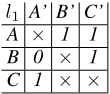
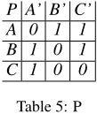
| l1 A' B' C' A × 1 1 B | l2 A' B' C' | P A' B' C' |
| A × 1 + | A 0 1 1 | |
| 0 × 1 | B 1 × + | B 1 0 1 |
| C 1 × × | C □ □× + ×□ | C 1 0 0 |
| Table 3: l1 | Table 4: l2 | Table 5: P |
to the "source" axis) contain only 0's. As such, they can be encoded with constraints l2 =⇒ ¬C and l2 =⇒ ¬C ′ .
When looking at table 5, we add the following constraints: A =⇒ ¬A′ , B =⇒ ¬B′ , C =⇒ ¬B′ and C =⇒ ¬C ′ .
After adding these constraints, only one 0 remains unblocked in the initial tables, which can be blocked with the following constraint: l1 ∧B =⇒ ¬A′ . So with this method we were able to encode the information using 6 binary constraints and 1 ternary constraint as opposed to 12 (the total number of 0's in the initial tables) ternary constraints.
4.3 Self-loops
In each factor, many labels may have no effect at all. A label l is irrelevant for factor Θk iff it has a self-loop transition in every state in Θk and no other transitions. All other labels are relevant. Among the relevant labels there are further labels that only have self-loop transitions, but not necessarily in every state. Encoding these labels as outlined so far, creates (with projection optimization) a clause lt ∧ sti =⇒ si+1 i for each state si in which l has a self-loop. These constraints are both repetitive and memory-inefficient, given that typically the majority of all labels is irrelevant for an individual factor.
To capture the semantics of self-loop transitions more compactly, we introduce an auxiliary variable SLtk :
- SLtk : Θk performed a self-loop transition at time t. We assert this semantic with the following constraint:
Let's now consider L→k = {l ∈ L | ∃(s, l, t) ∈ Tk s.t. s ̸= t}, i.e., the set of labels that include non-self-loop transitions in Θk, and L◦k = L \ L→k the labels that are only self-loops. If SLtk is false, i.e., the transition was not a self-loop, some label fromL→k was selected at timestep t (Eq. 15).
We cannot require that SLtk implies a disjunction of l ∈ L◦k as a label in L→k can have both self-loop and non-self-loop transitions. If a self-loop label l ∈ L◦k is executed, constraint 6 ensures that no label in L→k is executed and thus SLtk is true. Constraint 14 then enforces the self-loop. For relevant onlyself-loop labels (self-loops in some but not all states), we additionally need to ensure that they are executed in a state in which they have a self-loop via (both for time t and t + 1):
The transition semantics of labels l ∈ L→k is enforced as before. Since the semantics of labels l ∈ L◦k is encoded via constraint 16, we omit all constraints otherwise restricting their execution. We remove all primal containing lt and all dual constraints with lt on the left-hand side. If an l ∈ L◦k appears on the right-hand side of a projected dual clause, the clause specifies possible labels, e.g., in constraints of the type si =⇒ ∨ l. To replace these occurrences, we introduce a new SAT variable.
- NS tk : some label in L→k was executed.
We define its semantics using the constraints:
Note that ¬NS tk implies SLtk , but not vice versa - as labels may have both self-loop and non-self-loop transitions.
We replace all occurrences of l ∈ L◦k with ¬NS tk (and remove duplicates) stating that some self-loop can be performed while constraint 16 ensures that the selected self-loop is possible. For dual constraints where the right-hand-side are labels (i.e., source or target implies labels), there are almost always at least two possible labels as almost every state has a self-loop with an irrelevant label. To still enable the utilization of dual clauses in these cases, we generate them only if there is at most one relevant label on the right-hand-side. I.e. we may generate clauses of the form sti ⇒ lt ∨ ¬NS tk .
This encoding of self-loops introduces only two extra variables and 2|Sk| + |L◦k | + |L→k | + 2 constraints per transition system instead of |{L\L→k }| × |Sk|. Additionally, it lets us eliminate constraint 5. If no label is selected, SLtk must be true (constraint 15) and thus the states does not change (constraint 14). This ability is crucial when using more advanced methods for selecting horizon length (AlgorithmC, see [Rintanen, 2011] and Sec. 6) for satisficing planning.
| l1,l3 A' B' C' 0 0 | l2 A' B' C' 0 | l4 A' B' C' |
| A 1 | A 1 0 | A 0 1 0 |
| B 0 1 0 | B 0 0 0 | B 0 0 1 |
| C 0 0 1 Table 6: l1 and l3 | C 0 0 1 Table 7: l2 | C 0 0 0 Table 8: l4 |
Without the self-loop optimisation, we create constraints of the type l1 ∧ A =⇒ A′ for every state, for labels l1 and l3, and for label l2 we create the same type of constraint for every state where there is a self-loop plus constraints like l2 =⇒ ¬B (if using the projection optimisation) for every state where there is not a self-loop. Therefore, the number of clauses to encode self-loop transitions scales with O(|Sk||L◦ |).
With the self-loop optimisation we start by encoding the constraint A =⇒ (SL ⇐⇒ A′ ) for every state, for a total of 2|Sk| clauses. Then, we assert the preconditions of the relevant labels comprised only of self-loops, which in this case would be the constraint l2 =⇒ A′ ∨C ′ adding an extra |L◦ | clauses. Then, we add the constraint enforcing that if SL is false, then the transition executed was not a self-loop accounting for one constraint ¬SL =⇒ l4. Lastly, we include the constraints using the NS variable. This corresponds to NS =⇒ l4 for an additional clause and to ¬NS =⇒ ¬l4 for |L→k | additional clauses. So, we get O(|Sk| + |L|), which is often smaller than the encoding without the optimisation.
4.4 Label Groups
Similar to the optimization for self-loops, we can reduce redundancy in the encoding by exploiting the structure of label groups. Label groups are an optimisation for representing more compactly the transitions of each factor [Sievers, 2018]. This is based on the observation that oftentimes there are many labels that share the same set of transitions within a factor. For example, all irrelevant labels have a self-loop in every state. Therefore, a label group LG ⊆ L is a set of labels such that, for any l, l′ ∈ LG, (si, l, sj) ∈ Tk ⇐⇒ (si, l′ , sj) ∈ Tk. The same idea can be translated into the SAT encoding. In each factor, all labels within a given label group share the exact same set of transitions. As a result, encoding identical constraints for each label individually is inefficient. To avoid this duplication, we introduce one variable LGt per label group for each factor. Then the transition constraints can be encoded using label groups instead of labels. To maintain correctness across factors, we add an additional constraint that ensures a label can only be selected if its corresponding label group is also selected. Let LG be the set of all label groups in Θk. We then add for all LG ∈ LG the constraint LGt ⇔ ∨l∈LG lt .
| l1 | A' | B' | C' l2 A' | B' | C' |
| A | 0 | 1 | 1 A 0 | 1 | 1 |
| B | 0 | 0 | 1 B 0 | 0 | 1 |
| C | 1 Table | 0 9: | 0 l1 C 1 Table | 0 10: | 0 l2 |
Without the label group optimisation, the encoding of the constraints for the transitions of these two labels would be nearly identical, with the only difference in the constraints being the variable of the label, e.g., l1 ∧ A =⇒ ¬A′ and l2 ∧A =⇒ ¬A′ .
With the use of label groups, we can reduce all nearly identical constraints by introducing a new variable (LG) and a new constraint for each label group. With this new variable we can just encode the transitions using it, e.g., LG∧A =⇒ ¬A and assert that if a label group is being used, then at least one of its labels was selected: LG ⇔ l1 ∨ l2.
5 Parallelism
So far, our encoding has been restricted to generating sequential plans due to constraint 6, restricting us to at most one label per timestep. While this ensures correctness, it is highly limiting in practice, as it significantly increases the number of steps required to reach a solution (see e.g. [Kautz and Selman, 1996; Rintanen et al., 2006]). We show how to extend our encoding to support parallelism, i.e., selecting multiple labels simultaneously. Removing constraint 6 without additional restrictions could result in incorrect plans. There would be nothing to prevent labels from, e.g., executing transitions (si, l1, sj) and (si, l2, sj) concurrently in one factor, which may be invalid, e.g., if sj has no outgoing transitions.
We aim for a form of parallelism akin to the ∀-step parallelism for STRIPS and SAS+ tasks [Kautz and Selman, 1996; Rintanen et al., 2006]. In ∀-step parallelism, a set of actions can be applied in parallel if every linearisation is executable and leads to the same state. That is, if a1 and a2 are ∀-step parallel, then for any state s in which both are applicable, both ⟨a1, a2⟩ and ⟨a2, a1⟩ are valid and reach the same state.
We consider two different definitions, one of which is simpler to encode, and one that allows for more parallelism.
5.1 Self-loop Parallelism
Consider transitioning in some factor from state si to sj with a label l. Any label l′ that is a self-loop in both si and sj can be safely executed together with l in any order. We allow this parallelism only if l′ comprises only of self-loop transitions. That is, self-loop parallelism allows to execute at most one actual transition in each factor together with a set of self-loop only transitions. To enforce this, we replace constraint 6 with a new set of constraints 18, one per factor. These constraints ensure that at most one label from L→k is selected at each timestep.
However in the base encoding of the transition relation Tk, selecting two labels to be true requires both to be executed. This makes it impossible to execute a self-loop label l◦ together with a label ⃗l performing an actual transition: l◦ requires source and target state to be the same, while ⃗l requires them to be different. I.e. parallelism between two labels is only possible if both of them are self-loops in all factors.
Here we leverage the self-loop optimization. It enforces for each executed self-loop label l◦ only that both the source and the target state have a self-loop with l◦ (constraint 16). Source and target state must only be identical if no label from L→k is executed. Executing self-loops in parallel with one actual transition is still possible if SLtk is false.
Lastly, dualised constraints where the right-hand-side contains labels become critical, as they relied on at most one label being executed at each time. This will be a projected constraint of the from st(+1) i ⇒ ∨ lt with si either being a source or target state. Suppose a label l ∈ L→k would be executed that is impossible, i.e., not mentioned on the right-hand-side of the dualised constraint. Then no other l′ ∈ L→k can be selected for execution due to constraint 18. To satisfy the dualised constraint, the right-hand-side must contain ¬NS tk and NS tk must be false. But this forces via constraint 17 all non-self-loop-only labels to also be false, i.e. l must be false.
5.2 Chain Parallelism
Self-loop parallelism is by construction a subset of ∀-step parallelism: every set of actions A executable under self-loop parallelism is executable in parallel under ∀-step semantics.
As previously mentioned, labels that contain transitions of the form (si, l1, sj) and (si, l2, sj), should not be applied simultaneously. However, if both labels also allow for self-loop transitions at the target sj (i.e. (sj, l1, sj) and (sj, l2, sj)), then any ordering of the l1 and l2 is safe and leads to the same resulting state sj - with the idea that the label that is executed first transitions to sj and the other loops there.
This motivates a further notion of parallelism. We say that a set of labels L is executable under chains parallelism when transitioning from state si to state sj , if when we consider the non-self-loop labels L ∩ L→k , either |L ∩ L→k | = 1 or for all l ∈ L∩L→k the transition (sj, l, sj) exists.
We cannot simply allow or forbid a specific set of labels to be executed in parallel, since the validity of their parallel execution is dependent on sj. Let Lj be the set of labels which have a transition to state sj from another state. We need to encode that if some l ∈ Lj is executed all other l′ ∈ Lj \ {l} have a self-loop at sj. And thus if at least two are executed, all have a self-loop at sj. This exclusion is exactly the restriction that Rintanen et al.'s [2006] chains constraints describe - with Lj being the erasers and {l | l ∈ Lj and (sj, l, sj) ̸∈ Tk} being the requirers. For every factor Θk and target state sj we introduce 2|Lj| "helper" variables (hik,j and h′i k,j) along with constraints 19 to 22.
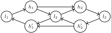
The core idea is the following: if a label l is selected and leads to state sj, then every other label that can transition to sj but lacks a self-loop at sj must be disabled. Figure 1 gives a visual idea behind the encoding. A normal edge represents an implication from the source to the target and a dashed edge represents an implication from the source to the negated target. Note that the dashed edges should only be present if the target does not contain a self-loop.
In contrast to self-loop parallelism, chains parallelism allows for executing two non-self-loop labels at the same time step. Thus moving from primal to dual constraints (see Sec. 4.1) is not sound any more, i.e., the dual constraints do not forbid all impossible transitions, (see counterexample in the appendix [Filipe et al., 2026b]) but only force that one of the selected labels is a possible transition. We therefore cannot omit primal constraints whenever we generate a dual constraint. As dual constraints provide useful information for unit-propagation, we nevertheless keep them. I.e. for chains parallelism we include both primal and dual constraints and only omit primal constraints 8, if there is a primal constraint 13 covering it.
Example 5. Consider labels l1 and l2 where they both have the transitions A- > B′ , A- > C ′ and C- > C ′ , but then only l2 has the transition B- > B′ .
| l1 | A' | B' | C' |
| A | 0 | 1 | 1 |
| B | 0 | 0 | 0 |
| C | 0 | 0 | 1 |
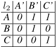
From our encoding, these two labels can only be executed together under ∀-step parallelism if they are moving to state C ′ . Let's see why: For starters, for both labels to even have the possibility of being executed at the same time, their preconditions have to be satisfied, which means we are either starting at A or at C since l1 is not executable in B. If we start at A and try to move to B′ , then the chains for this state would generate the constraints: l1 ∧ B′ =⇒ h1, l2 ∧ B′ =⇒ h′1 and h′1 =⇒ ¬l1, thus making it impossible to select both l1 and l2 while moving to B′ , which is the intended behaviour since not all linearisations are possible, e.g., it is not possible to execute the labels in the order l2, l1 since l1 does not have a self-loop at B′ . Then if we were to move to state C ′ , we would only require the constraints l1 ∧ C ′ =⇒ h1 and l2 ∧ C ′ =⇒ h′1 from the chains corresponding to this state, as the constraint h′1 =⇒ ¬l1 would no longer be generated since l1 has a self-loop at C ′ , thus making it possible to execute both labels in parallel when moving from A to C ′ . If we were to try to move from C to C ′ exactly the same constraints would be generated since once again both labels have a self-loop at the target.
This means that in total there are only 4 ways in which these labels can be executed in parallel: (A, l1, C ′ ), (C, l2, C ′ ), (A, l2, C ′ ), (C, l1, C ′ ), (C, l1, C ′ ), (C, l2, C ′ ) and (C, l2, C ′ ), (C, l1, C ′ ).
Theorem1. If a set of labels L is executable in parallel under chains parallelism then they are ∀-step parallel.
Proof. Suppose L is executable in parallel under chains parallelism. Let ⃗L be an arbitrary ordering of L and we have to prove that ⃗L is executable and all linearisiations of L yield the same state. ⃗L is executable if it is executable for every individual factor. Consider an arbitrary one. Any label l ∈ L∩L◦ does not change the state and can be executed at any position and thus be ignored. Observe that the remaining actions perform overall a single state transition from state si to state sj. In the execution of ⃗L, the first label l ∈ ⃗L \ L◦ can (as enforced by the primal and dual constraints) and will perform the transition. Given constraints 19 to 22, either |L \ L◦ | = 1 or all other l′ ∈ ⃗L \ L◦ have a self-loop at sj allowing them to be executed and that execution leading to sj .
5.3 FTS Parallelism vs ∀-step Parallelism
Next, we study the relation of self-loop and chains parallelism with classical ∀-step parallelism on FTS and SAS+ tasks.
Consider how SAS+ tasks are compiled into FTS tasks. In SAS+ tasks actions are specified via preconditions and effects, which are (partial) variable assignments. When translated into FTS, each variable corresponds to a factor (the atomic projection over that variable) and each action corresponds to a label. Thus, the transitions for label l in Θk belong to one of four cases, depending of whether the value of the variable k is defined for the preconditions and effects:
- vk ̸∈ pre(l), vk ̸∈ eff (l): there is a self-loop on all states in Θk
- vk ∈ pre(l), vk ̸∈ eff (l): there is a single self-loop transition (pre(l)[k], l, pre(l)[k])
- vk ̸∈ pre(l), vk ∈ eff (l): there are transitions (s, l, eff (l)[k]) from each s ∈ Θk
- vk ∈ pre(l), vk ∈ eff (l): there is a single transition (pre(l)[k], l, eff (l)[k])
Self-loop parallelism is provably weaker than regular ∀-step parallelism. Consider an SAS+ problem with two actions a1 and a2 so that a1 has the effects v1 = 1 and v2 = 2, while a2 has v2 = 2 and v3 = 3. None of the actions have preconditions. a1 and a2 can clearly be executed in any order and all such orders lead to the same state. However w.r.t. the variable v2 none of the two actions is a self-loop and thus only one of them can be executed in parallel in our encoding.
However, chains parallelism is a generalisation of the ∀- step parallelism on SAS+ tasks.
Theorem 2. Consider a FTS task whose factors are atomic projections of a SAS+ task. Then, if L is executable in parallel under the classical ∀-step parallelism, it is also executable under chains parallelism.
Proof. Let L be a set of labels executable under ∀-step parallelism. We can again ignore all irrelevant labels and focus on a single factor. We consider transitioning from state si to state sj (if si = sj all executed transitions for that factor are self-loops, trivialising the conditions). Let l ∈ L be an executed relevant label. There are linearisations of L in which l is the first label and one in which l is the last label. From the latter case, we know that there must be a transition for l ending at sj (either from si or a self-loop). From the former, we know that there is a transition for l that starts at si (either a self-loop at si or transitioning to sj). If l is a self-loop in both si and sj, then l is a self-loop in all states if this factor is an atomic projection from a SAS+ problem. Otherwise l must have a transition (si, l, sj). Suppose it does not have the transition (sj, l, sj). If this is the only non-self-loop label for the factor, no problem arises. Otherwise, there must be another label l′ for which the same reasoning holds. Then both ll′ and l′ l must be executable and reach the state sj. Note that it is impossible for l to have the transition (si, l, si) - as in the SAS+ sense it has an effect moving it to sj. The same holds for l′ , thus if executed, l′ forces a transition to sj - as it cannot loop at si. Since l′ l must be executable due to ∀-step parallelism, l must be able to loop at sj, thus forcing the transition (sj , l, sj ), which satisfies the chains-parallelism condition.
6 Experiments
We implemented our encodings on FTSPlan [Torralba et al., 2023], and ran experiments on all International Planning Competition domains, containing in total 2026 instances. We also ran experiments on the FTS benchmark which contains a total of 431 instances. A snapshot of the data and code used is archived at [Filipe et al., 2026a]. The experiments were run using Lab [Seipp et al., 2017] on an AMD EPYC 9654 with a memory limit of 1.75GB and a time limit of 1800 seconds. Our encodings use the Kissat SAT solver [Biere et al., 2024]. Madagascar comes with its own solver specifically tailored to its encoding and inextricably linked to it, as such it was ran with it.
| One-by-One | AlgC | |||||
|---|---|---|---|---|---|---|
| Seq | S-L | Chains | Seq | S-L | Chains | |
| Baseline | 603 | - | - | 764 | - | - |
| SL | 659 | 985 | 1096 | 1097 | 1270 | 1271 |
| SL+LG | 668 | 1001 | 1116 | 1014 | 1221 | 1271 |
| SL+P | 708 | 1080 | 1196 | 1219 | 1418 | 1431 |
| SL+P+LG | 712 | 1065 | 1184 | 1113 | 1336 | 1393 |
| SAT | FF | MpC | |||||
|---|---|---|---|---|---|---|---|
| Seq | S-L | Chains | - | p.o. | ∀ | ∃ | |
| None | 979 | 1236 | 1288 | 1318 | 1615 | 1368 | 1431 |
| LR | 1095 | 1338 | 1344 | 1324 | 1596 | - | - |
| LR+S | 1219 | 1418 | 1431 | 1430 | 1627 | - | - |
| LR+S+M | 1039 | 1241 | 1210 | 1314 | 1537 | - | - |
We conducted two sets of experiments using a modified version of Fast Downward [Helmert, 2006] which supports the FTS representation (except for Madagascar) to evaluate our strategies. The first set (Table 13) uses the transformations label reduction (LR) and shrinking (S) and presents the results of the baseline encoding (which encodes transitions only using constraint 7) as well as the results of encodings using projections (P), self-loop (SL) and label grouping (LG) optimisations with different parallelism strategies (Seq, for no parallelism; S-L for Self-loop parallelism; Chains for Chains parallelism) as well as different strategies for formula generation (One-by-One for generating a new formula with a length increased by 1 regarding the previous formula when that one is proved unsatisfiable; AlgC, similar to what is proposed by [Rintanen, 2014]). The second set (Table 14) explores the effect of applying various task transformations on top of the best-performing configuration, allowing us to better understand their impact. For reference, we also include the performance of the state-of-the-art SAT-based planner Madagascar (MpC), which was ran with configurations for ∀ and ∃- step parallelism combined with AlgC formula generations, as well as an adapted version of the FF heuristics [Hoffmann and Nebel, 2001] [Torralba and Sievers, 2019] with lazy-greedy search with and without preferred operators (p.o.). This latter configuration is equivalent to what is commonly known as FTSPlan [Torralba et al., 2023]. Due to the large number of domains, we report only the total number of solved instances. An appendix is available [Filipe et al., 2026b] with detailed results per domain as well as a more in depth analysis of the impact of each individual projection.
Parallelism and Formula Generation Table 13 highlights the performance differences across various encoding strategies. Sequential encodings significantly underperform encodings that support parallelism, solving around 300 fewer instances, since they require more timesteps to find a satisfying assignment. As a new formula is generated for each timestep, this results in more formulas being attempted and, consequently, an increase in required solving time. When comparing the two parallelism strategies, chain-based parallelism outperforms the self-loop-based approach, despite requiring additional variables and clauses. This indicates that the benefit of reducing the number of timesteps, and thus the number of formulas that must be solved, outweighs the cost introduced by the more complex encoding. Regarding formula generation strategies, encodings using the One-by-One approach significantly underperform, regardless of optimisations, compared to AlgC, solving 200-400 fewer instances. This is due to the requirement to prove unsatisfiability for each formula length before proceeding to the next, which becomes increasingly costly for longer plans.
Optimisations The projection optimisation, which reduces the number of constraints and their arity, shows a consistent improvement across configurations, solving 50 to 200 more instances. On the other hand, the label groups optimisation seems to have a negative impact. Aside from one result in One-by-One, the use of this optimisation always reduced the number of instances solved indicating that the introduction of the additional variable as well as the new overhead in the formula ends up being more harmful than beneficial. Regarding the Self-loop optimisation, we only present the baseline results without it because it would not be possible to allow any sort of relevant parallelism without this optimisation as otherwise the base constraint encoding the transitions would be too restrictive.
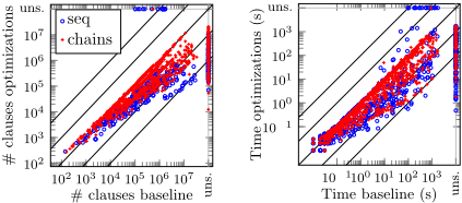
Figure 2 shows the difference in formula size (in terms of the number of clauses) and total time with and without using the projection optimisation. Using chains, with the optimisation enabled, the encoding produces less clauses for a total of 533 tasks while only exceeding the number of clauses for 299. Additionally, it can also be seen that the difference in the number of clauses in the cases where it produces less clauses is much bigger than in the cases where it produces more. We do not provide an analysis for the self-loop optimisation because it has to be enabled in order for parallelism to be allowed. We also do not provide a plot to analyse how the number of variables changes with each optimisation since the number of variables introduced by them is negligible.
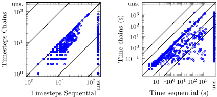
Figure 3 shows the impact of parallelism in more detail. In this case, the main difference is in reducing the number of time steps necessary to find a plan. This translates into a very significant difference in terms of time, sometimes of several orders of magnitude. This is not surprising because the SAT formula grows linearly with the number of time steps, but solving the larger formulas can be exponentially harder.
Transformations When analysing the impact of transformations, it is clear that they can influence performance, both positively and negatively. While our default set of transformations consistently achieves the best results, merge (M) transformations consistently decrease performance, sometimes even falling below the encoding without any transformations. We evaluated the merge strategies available in FTSPlan, namely DFP and MIASM, setting a maximum factor size of 100. MIASM obtained slightly better results than DFP (around 5% higher coverage) and is the configuration reported as M in the paper. Coverage was lower or equal in every single domain compared to encodings not using merging. This drop can be attributed to two key factors.
The first is the loss of parallelism. Merging transition systems can force previously independent labels to be treated as interdependent. For example, imagine two transition systems and two labels: one label is only relevant in the first system, and the other only in the second. After merging, both labels become relevant in the combined system and may even collapse into a single label during label reduction. As a result, they can no longer be executed in parallel, leading to longer plans with more timesteps.
The second issue is the increase in state space. When multiple systems are merged, the combined system may contain many more states than each system individually. This expansion leads to a corresponding increase in the number of possible transitions that must be encoded, thus increasing the overall size and complexity of the formula.
Notably, these merge strategies were originally devised for computing heuristics rather than for problem reformulation. In the former setting, merging typically continues until all variables have been merged, while for the latter setting it is arguably more important to decide if merging is useful at all. Other merge strategies from the literature are likely to run into the same issues for this reason. While setting a size limit, as done in FTSPlan and here, provides a practical safeguard, devising merge strategies specifically tailored to task reformulation remains an open problem and is beyond the scope of this paper.
| FF | SAT | |||||
|---|---|---|---|---|---|---|
| Σ | - | (p.o.) | Chains | Seq | S-L | |
| burnt-pancakes | 100 | 60 | 63 | 48 | 54 | 55 |
| matrix-mult | 11 | 11 | 11 | 11 | 11 | 11 |
| cavediving-adl14 | 20 | 7 | 7 | 8 | 7 | 8 |
| pancakes | 100 | 58 | 66 | 53 | 58 | 63 |
| rubiks-cube | 100 | 9 | 10 | 45 | 47 | 47 |
| topspin | 100 | 22 | 22 | 29 | 30 | 28 |
| Σ | 431 | 167 | 179 | 194 | 207 | 212 |
FTS Benchmark Table 15 presents the results of running FF (with and without preferred operators) and our encodings on the FTS Benchmark using label reduction and shrinking. It can be seen that just like in the International Planning Competition Benchmark (IPC), the inclusion of the projections always has a positive impact. However, there are two key differences to the results of the IPC. The first is that now our encodings outperform FF both with and without preferred operators. The second is that the encoding using chains parallelism, achieves the worst results among our encodings. This is due to the fact that in this benchmark there is almost no parallelism allowed, and as such we cannot find significantly shorter plans using the encodings that support parallelism. So, in this scenario the chains encoding mostly only introduces the additional overhead of the extra variables and constraints, without any benefits. Note, however, that the lack of parallelism in this benchmark is not directly related to whether the input task is in SAS+ or FTS representation, so one should not conclude that paralellism is irrelevant in this setting. This is simply due to it being a relatively small benchmark set compared to the IPC and consisting mostly of permutation puzzles who typically lack parallelism compared to planning tasks where multiple agents/components can perform actions simultaneously.
7 Conclusions
We presented several SAT encodings for Factored Transition Systems (FTS), including techniques leveraging projections, self-loops, label groups, and different forms of parallelism. Empirically, we have shown that our encoding matches the state-of-the-art SAT-based planner Madagascar in total instances solved in the IPC benchmark even though we do not support ∃-step parallelism. In the IPC benchmark, we also outperform FF without preferred operators while in the FTS benchmark, we outperform FF both with and without preferred operators.
For future work, we aim to further relax the constraints on parallelism, to support ∃-step parallelism. Additionally, exploring new merge strategies tailored for SAT encodings could help avoid the problems of existing merging strategies.
Acknowledgements
This publication is part of the project "Exploiting Problem Structures in SAT-based Planning" with file number OCENW.M.22.050 of the research programme Open Competition which is financed by the Dutch Research Council (NWO).
@inproceedings{ijcai2026p249,
  title     = {Transforming and Encoding FTS for SAT Solving: What Helps, What Hurts},
  author    = {Filipe, João and Torralba, Álvaro and Behnke, Gregor},
  booktitle = {Proceedings of the Thirty-Fifth International Joint Conference on
               Artificial Intelligence, {IJCAI-26}},
  publisher = {International Joint Conferences on Artificial Intelligence Organization},
  editor    = {Diego Calvanese},
  pages     = {2236--2246},
  year      = {2026},
  month     = {8},
  note      = {Main Track},
  doi       = {10.24963/ijcai.2026/249},
  url       = {https://doi.org/10.24963/ijcai.2026/249},
}
TY - CPAPER TI - Transforming and Encoding FTS for SAT Solving: What Helps, What Hurts AU - Filipe, João AU - Torralba, Álvaro AU - Behnke, Gregor T2 - Proceedings of the Thirty-Fifth International Joint Conference on Artificial Intelligence, IJCAI-26 PB - International Joint Conferences on Artificial Intelligence Organization PY - 2026 SP - 2236 EP - 2246 DO - 10.24963/ijcai.2026/249 UR - https://doi.org/10.24963/ijcai.2026/249 ER -Copied
Machine-readable versions of this paper, for tools and AI agents:





