
CMACE: CMAES-based Counterfactual Explanations for Black-box Models
Proceedings of the Thirty-Third International Joint Conference on Artificial Intelligence. Main Track. Pages 539-547.
https://doi.org/10.24963/ijcai.2024/60
Keywords
- Machine Learning: ML: Optimization
- AI Ethics, Trust, Fairness: ETF: Trustworthy AI
- AI Ethics, Trust, Fairness: ETF: Explainability and interpretability
- Machine Learning: ML: Trustworthy machine learning
Abstract
Explanatory Artificial Intelligence plays a vital role in machine learning, due to its widespread application in decision-making scenarios, e.g., credit lending. Counterfactual Explanation (CFE) is a new kind of explanatory method that involves asking “what if ”, i.e. what would have happened if model inputs slightly change. To answer the question, Counterfactual Explanation aims at finding a minimum perturbation in model inputs leading to a different model decision. Compared with model-agnostic approaches, model-specific CFE approaches designed only for specific type of models usually have better performance in finding optimal counterfactual perturbations, owing to access to the inner workings of models. To deal with this dilemma, this work first proposes CMAES-based Counterfactual Explanations (CMACE): an effective model-agnostic counterfactual generating approach based on Covariance Matrix Adaptation Evolution Strategy (CMA-ES) and a warm starting scheme that provides good initialization of the counterfactual's mean and covariance parameters for CMA-ES taking advantage of prior information of training samples. CMACE significantly outperforms another state-of-art (SOTA) model-agnostic approach (Bayesian Counterfactual Generator, BayCon) with various experimental settings. Extensive experiments also demonstrate that CMACE is superior to a SOTA model-specific approach (Flexible Optimizable Counterfactual Explanations for Tree Ensembles, FOCUS) that is designed for tree-based models using gradient-based optimization.
- [Wachter et al., 2017] Sandra Wachter, Brent Mittelstadt, Christo- pher Russell. Counterfactual Explanations without Opening the Black Box: Automated Decisions and the GDPR. In Harvard Journal of Law and Technology, 2017.
- [Tolomei et al., 2017] Gabriele Tolomei, Fabrizio Silvestri, Andrew Haines, and Mounia Lalmas. Interpretable Predictions of Tree- Based Ensembles via Actionable Feature Tweaking. In Interna- tional Conference on Knowledge Discovery and Data Mining, 2017.
- [Lucic et al., 2022] Ana Lucic, Harrie Oosterhuis, Hinda Haned, and Maarten de Rijke. FOCUS: Flexible Optimizable Counter- factual Explanations for Tree Ensembles. In AAAI Conference on Artificial Intelligence. 2022.
- [Kanamori et al., 2020] Kentaro Kanamori, Takuya Takagi, Ken Kobayashi, and Hiroki Arimura. DACE: Distribution-Aware Counterfactual Explanation by Mixed-Integer Linear Optimiza- tion. In International Joint Conference on Artificial Intelligence, 2020. IJCAI
- [Carreira-Perpinan and Hada, 2021] Miguel A Carreira-Perpinan, and Suryabhan Singh Hada. Counterfactual Explanations for Oblique Decision Trees: Exact, Efficient Algorithms. In AAAI Conference on Artificial Intelligence. 2021.
- [Parmentier and Vidal, 2021] Axel Parmentier, and Thibaut Vidal. Optimal Counterfactual Explanations in Tree Ensembles. In In- ternational Conference on Machine Learning. 2021.
- [Kanamori, et al., 2021] Kentaro Kanamori, Takuya Takagi, Ken Kobayashi, Yuichi Ike, Kento Uemura, and Hiroki Arimura. Or- dered Counterfactual Explanation By Mixed-Integer Linear Op- timization. In AAAI Conference on Artificial Intelligence. 2021.
- [Dandl et al., 2020] Susanne Dandl, Christoph Molnar, Martin Binder, and Bernd Bischl. Multi-objective counterfactual expla- nations. In International Conference on Parallel Problem Solv- ing from Nature, 2020.
- [Romashov et al., 2022] Piotr Romashov, Martin Gjoreski, Kacper Sokol, Maria Vanina Martinez, and Marc Langheinrich. Bay- Con: Model-agnostic Bayesian Counterfactual Generator. In In- ternational Joint Conference on Artificial Intelligence, 2022.
- [Hansen, 2016] Nikolaus Hansen. Hansen, N. 2016. The CMA Evolution Strategy: A Tutorial. In arXiv preprint arXiv:1604.00772.
- [Hansen et al.,2019] Nikolaus Hansen, Youhei Akimoto, and Petr Baudis. CMA-ES/pycma on Github. . In Zenodo. DOI:10.5281/zenodo.2559634. 2019. DOI
- [Verma et al., 2022] Sahil Verma, Varich Boonsanong, Minh Hoang, Keegan E. Hines, John P. Dickerson, and Chirag Shah. Counterfactual Explanations and Algorithmic Recourses for Machine Learning: A Review. In arXiv preprint arXiv. 2022.
- [Krause et al., 2016] Oswin Krause, Dídac Rodríguez Arbonès, and Christian Igel. CMA-ES with Optimal Covariance Update and Storage Complexity. In Advances in Neural Information Pro- cessing Systems, 2016.
- [Hamano et al., 2022] Ryoki Hamano, Shota Saito, Masahiro No- mura, and Shinichi Shirakawa. CMA-ES with Margin: Lower- Bounding Marginal Probability for Mixed-Integer Black-Box Optimization. In Annual Conference on Genetic and Evolution- ary Computation. 2022.
- [Nomura et al., 2021] Masahiro Nomura, Shuhei Watanabe, Youhei Akimoto, Yoshihiko Ozaki, and Masaki Onishi. Warm Starting CMA-ES For Hyperparameter Optimization. In AAAI Confer- ence on Artificial Intelligence. 2021.
- [Feurer et al., 2015] Matthias Feurer, Jost Tobias Springenberg, and Frank Hutter. Initializing Bayesian Hyperparameter Optimiza- tion Via Meta-Learning. In AAAI Conference on Artificial Intel- ligence. 2015.
- [Perrone et al., 2018] Valerio Perrone, Rodolphe Jenatton, Matthias Seeger, Cédric Archambeau. Scalable Hyperparameter Transfer Learning. In Advances in Neural Information Processing Sys- tems. 2018.
- [Perrone et al., 2019] Valerio Perrone, Huibin Shen, Matthias Seeger, Cedric Archambeau, Rodolphe Jenatton. Scalable Hy- perparameter Transfer Learning. In Advances in Neural Infor- mation Processing Systems. 2018. Learning search spaces for Bayesian optimization: Another view of hyperparameter trans- fer learning. In Advances in Neural Information Processing Sys- tems. 2019.
- [Ash and Adams, 2019] Jordan T. Ash, and Ryan P. Adams. On the Difficulty of Warm-Starting Neural Network Training. In Ad- vances in Neural Information Processing Systems. 2019.
- [Chu et al., 2015] Bo-Yu Chu, Chia-Hua Ho, Cheng-Hao Tsai, Chieh-Yen Lin, and Chih-Jen Lin. Warm Start for Parameter Selection of Linear Classifiers. In ACM SIGKDD Conference on Knowledge Discovery and Data Mining. 2015.
- [Loshchilov and Hutter, 2017] Ilya Loshchilov, and Frank Hutter. Sgdr: Stochastic gradient descent with warm restarts. In Inter- national Conference on Learning Representations. 2017.
- [Snoek et al., 2012] Jasper Snoek, Hugo Larochelle, and Ryan Prescott Adams. Practical Bayesian Optimization of Machine Learning Algorithms. In Advances in Neural Information Pro- cessing Systems. 2012.
- [Wang et al., 2013] Ziyu Wang, Masrour Zoghi, Frank Hutter, David Matheson, and Nando De Freitas. Bayesian optimization in high dimensions via random embeddings. In International Joint Conference on Artificial Intelligence. 2013. IJCAI
- [Springenberg et al., 2016] Jost Tobias Springenberg, Aaron Klein, Stefan Falkner, and Frank Hutter. Bayesian Optimization with Robust Bayesian Neural Networks. In Advances in Neural In- formation Processing Systems. 2016.
- [Lindauer et al., 2022] Marius Lindauer, Katharina Eggensperger, Matthias Feurer, André Biedenkapp, Difan Deng, Carolin Ben- jamins, René Sass, and Frank Hutter. SMAC3: A Versatile Bayesian Optimization Package for Hyperparameter Optimiza- tion. In Journal of Machine Learning Research. 2022. [Miller, 2019]
- Tim Miller. 2019. Explanation in artificial intelli- gence: Insights from the social sciences. In Artificial Intelli- gence. 2019.
- [Naumann and Ntoutsi, 2021] Philip Naumann, and Eirini Ntoutsi. Consequence-Aware Sequential Counterfactual Generation. In European Conference on Machine Learning. 2021.
- [Albini et al., 2020] Emanuele Albini, Antonio Rago, Pietro Ba- roni, and Francesca Toni. Relation-Based Counterfactual Expla- nations for Bayesian Network Classifiers. In International Joint Conference on Artificial Intelligence. 2020. IJCAI
- [Cheng et al., 2021] Furui Cheng, Yao Ming, and Huamin Qu. DECE: Decision Explorer with Counterfactual Explanations for Machine Learning Models. In IEEE Transactions on Visualiza- tion and Computer Graphics. 2021.
- [Kenny and Keane, 2021] Eoin M. Kenny, and Mark T. Keane. On Generating Plausible Counterfactual And Semi-Factual Expla- nations For Deep Learning In AAAI Conference on Artificial In- telligence. 2021.
- [Olson et al., 2021] Matthew L. Olson, Roli Khanna, Lawrence Neal, Fuxin Li, and Weng-Keen Wong. Counterfactual state ex- planations for reinforcement learning agents via generative deep learning. In Artificial Intelligence. 2021.
- [Tsirtsis et al., 2021] Stratis Tsirtsis, Abir De, and Manuel Gomez- Rodriguez. Counterfactual Explanations in Sequential Decision Making Under Uncertainty. In Advances in Neural Information Processing Systems. 2021.
- [Galhotra et al., 2021] Sainyam Galhotra, Romila Pradhan, and Babak Salimi. Explaining Black-Box Algorithms Using Prob- abilistic Contrastive Counterfactuals. In ACM SIGMOD Con- ference. 2021.
- [Yang et al., 2021] Fan Yang, Sahan Suresh Alva, Jiahao Chen, and Xia Hu. Model-Based Counterfactual Synthesizer for Interpre- tation. In SIGKDD Conference on Knowledge Discovery and Data Mining. 2021.
- [Augustin et al., 2022] Maximilian Augustin, Valentyn Boreiko, Francesco Croce, and Matthias Hein. Diffusion Visual Counter- factual Explanations. In Advances in Neural Information Pro- cessing Systems. 2022.
References were extracted automatically from the PDF and may contain errors.
Full text extracted automatically from the PDF; figures, tables and equations may differ. The PDF is the version of record.
1 Introduction
The development of Machine Learning (ML) has brought ubiquitous opportunities in science and technology analytics. However, ML models are black boxes for users in many scenarios and lack of interpretability. Except for prediction accuracy, there are increasing demands for model interpretability in decision-making or risk-sensitive scenarios. Specifically, General Data Protection Regulation (GDPR) protects fundamental rights and freedoms of natural persons to request an explanation of any decision made by the machine, and thus further emphasize the significance of Explainable Artificial Intelligence (XAI). As one of the emerging techniques under the umbrella of XAI, Counterfactual Explanations (CFE) provide explanations by exploring potential outcomes that would have occurred if the inputs are changed. CFE enables users to understand what needs to change in order to get a predefined outcome, which makes it an effective tool for examining the influence of small perturbations on model output.
*Corresponding authors
Since CFE is able to explain how feature perturbations would affect outcomes, it is particularly valuable to risksensitive scenarios, such as financial credit service and medical treatment, in which decisions made by models may cause great impact on human or society. For instance, a rejected loan applicant may want to know how to alter his/her information to meet the regulations. In this case, CFE can provide effective suggestions and may help the applicant to have the application accepted.
Therefore, identifying the optimal CFE and providing persuasive suggestions for users to make subsequent decisions are essential. Wachter et al. [Wachter et al., 2017] first formulated CFE as an optimization problem. The optimization goal of generating a counterfactual is to minimize the distance between the counterfactuals and the original instance (L1/L2 distance, etc.) while satisfying the constraint that the output of the classifier model changes to a different result or desired class. The authors also proposed an alternative formulation of the minimization problem for generating counterfactuals in gradient-based differentiable models. In this formulation, the loss function is defined as a weighted sum of two terms: one is the distance loss between the counterfactuals and the original instance, while the other is the distance loss between the model's prediction and the desired class.
Subsequent studies [Albini et al., 2020; Cheng et al., 2021; Kenny and Keane, 2021; Olson et al., 2021; Tsirtsis et al., 2021; Galhotra et al., 2021; Yang et al., 2021] predominantly adopted either of the aforementioned problem definitions when generating counterfactuals. While gradient-based approaches [Cheng et al., 2021; Kenny and Keane, 2021; Olson et al., 2021; Augustin et al., 2022] are only appli-
Algorithm 1 CMACE
Input: a trained black-box binary classification model M(x), training samples X, an instance to be explained x Output: counterfactual perturbations
˙x∗ 1: initialize: m0, C0 =WarmStarting(x,X) 2: for g = 1 to N do 3: ˙xg,1:λ = Sampling(mg-1, Cg-1) 4: Evaluate ℓg,1:λ = ℓ (x, ˙xg,1:λ|M) 5: mg = SelectionRecombination( ˙xg,1:λ, ℓg,1:λ) 6: Cg = CovarianceMatrixAdaptation(mg, ˙xg,1:λ, ℓg,1:λ) 7: Store ℓ∗g =min {ℓ∗g-1 , ℓ∗g,1:λ} and corresponding ˙x∗g 8: if (a satisfying solution is found) then 9: Break 10: end if 11: end for 12: return ˙x∗cable to differentiable models, there remains a gap in addressing non-differentiable models such as tree ensembles and SVMs. Existing gradient descent algorithms fail to obtain counterfactuals for these models. In recent years, numerous studies have attempted to tackle this issue through either model-specific approaches tailored for specific types of models or model-agnostic heuristic approaches. Compared to model-agnostic methods that are not limited by specific model types, model-specific CFE approaches generally exhibit superior performance in identifying optimal counterfactual perturbations due to their access to the internal mechanisms of the models.
To address the limitations of both model-specific and model-agnostic approaches, we propose CMAES-based Counterfactual Explanations (CMACE): a highly effective model-agnostic counterfactual explanation approach based on Covariance Matrix Adaptation Evolution Strategy (CMAES) [Hansen, 2016; Hansen et al.,2019]. To the best of our knowledge, this is the first counterfactual generation approach based on CMA-ES-an excellent optimizer specialized in solving difficult non-linear, non-convex, and blackbox optimization problems-ensuring optimality of generated counterfactuals. Additionally, to improve optimization performance, we introduce a warm starting scheme that leverages prior information from training samples to provide good initialization of mean and covariance parameters for CMA-ES. Through extensive experimentation involving four datasets and six models with different distance functions adopted, CMACE demonstrates superiority over stateof-the-art (SOTA) model-specific approach FOCUS (Flexible Optimizable Counterfactual Explanations for Tree Ensembles) designed for tree-based models using gradient-based optimization, as well as outperforms another SOTA modelagnostic approach BayCon (Bayesian Counterfactual Generator) based on Bayesian optimization.
2 RelatedWork
Since the concept of CFE is introduced [Wachter et al., 2017], numerous studies have emerged [Verma et al., 2022].
For differentiable models, gradients of counterfactuals can be computed with gradient descent algorithms. While non-differentiable models require solver-based approaches [Kanamori et al., 2020; Carreira-Perpinan and Hada, 2021; Parmentier and Vidal, 2021; Kanamori, et al., 2021] that formulate CFE as a mixed-integer linear optimization (MILO) problem for additive classifiers. This approach is applicable only to linear or piece-wise linear models such as tree ensemble and linear models since it requires complete access to internal model information used in generating counterfactuals. And thus, these types of models are considered white-box.
Another research area in CFE for non-differentiable models primarily focuses on model-specific approaches and tree ensemble models [Wachter et al., 2017; Tolomei et al., 2017; Lucic et al., 2022]. As these approaches are model-specific, the resulting counterfactuals are naturally superior to other methods not tailored for tree ensemble models. Tolomei et al. [Tolomei et al., 2017] proposed a feature tweaking (FT) algorithm that enumerates alternative paths in each tree to alter the ensemble decision. While this method provides useful counterfactual explanations in various applications, it does not always produce optimal (or even feasible) counterfactual explanations for tree ensembles since perturbing examples may not necessarily result in counterfactual examples. Recently, Lucic et al. [Lucic et al., 2022] introduced FOCUS as a model-specific CFE approach suitable for tree ensembles that achieves state-of-the-art performance in generating valid and distance-minimized counterfactuals. FOCUS adopts a tree approximation with differentiable sigmoid functions and can be formulated as a gradient-based minimization problem with guaranteed validity of generated counterfactuals and minimized distances from original instances. Extensive experiments demonstrate that FOCUS outperforms FT and DACE [Wachter et al., 2017], another MILO solver-based approach, regarding both validity of counterfactuals and distances to original instances across all experiment settings.
While model-specific CFE approaches generally significantly superior performance compared to their modelagnostic counterparts, the latter are more suitable for realworld industry applications because they require fewer assumptions or restrictions on underlying models. With increasing demand for model agnosticity in counterfactual explanations, significant progress has been made in modelagnostic CFE approaches. State-of-the-art studies include: Multi-objective Counterfactual Explanations (MOC, [Dandl et al., 2020]), which formulates counterfactual generation as a multi-objective optimization problem solved with genetic algorithms; Bayesian Counterfactual Generator (BayCon, [Romashov et al., 2022]), which is based on Bayesian optimization [Snoek et al., 2012; Wang et al., 2013; Springenberg et al., 2016; Lindauer et al., 2022] and guarantees good effectiveness in generating counterfactuals due to its top-ranking optimization performance in domains of black-box model optimization. Bayesian optimization leverages prior information on model inputs and outputs to guide the sampling distribution and search direction of subsequent steps following Bayes' theorem. In comparative experiments, BayCon outperforms other approaches such as MOC in generating highquality counterfactual explanations with respect to distance from original instances. Therefore, it can be considered a top-tier model-agnostic approach for counterfactual explanation.
| Dataset | Features | Train Samples | Test Samples |
|---|---|---|---|
| Heloc | 23 | 7,321 | 3,138 |
| Wine | 11 | 3,428 | 1,470 |
| Compas | 6 | 4,320 | 1,852 |
| Shopping | 9 | 8,631 | 3,699 |
3 Methodology
In this section, we elaborate the methodology of CMACE, the counterfactual explanation approach based on CMA-ES and a warm starting initialization scheme for counterfactuals. CMA-ES is an excellent optimizer that has gained increasingly applications in recent years owing to its effectiveness for solving difficult non-linear, non-convex and black-box optimization problems. CMA-ES incorporates the concept of covariance matrix adaptation into domains of evolutionary computations to improve the effectiveness and efficacy of optimal search process. It carries out the optimization procedure by sampling from a multivariate Gaussian distribution (MGD), ranking the sampled points according to their objective function values, and iteratively updating the mean and covariance parameters of MGD based on the ranked points. The main search procedure of CMA-ES can be generalized as followings.
Firstly, a population of λ search points (individuals) are sampled from a MGD, specifically, for generation number g = 0, 1, 2, . . ., the sampling equation of k-th individual is formulated as
where σg is the step-size (i.e. the "overall scale" or standard deviation of the distribution), mg is the mean parameters of MGD and C g is the covariance matrix of MGD, these parameters of MGD would be updated iteratively through the following adaption steps.
Secondly, the mean vector of individuals is updated through selection and recombination:
where xg+1 i:λ is i-th best individual of generation g+1 of sampling (Eq. (1)), and wi=1,...,µ are positive weight coefficients for recombination (∑µi=1 wi = 1, w1 ≥ w2 ≥ ... ≥ wµ > 0).
Then the step-size σg is updated by adpating a step-size cumulation path:
where cσ and dσ denote decay rate of evolution path for the step-size and damping parameter scaling the change magnitude for σ.
Lastly, covariance matrix adaptation (CMA) of MGD for generation g+1 is formulated through updating a covariancematrix cumulation path pg+1 c :
where ccov and µcov denote learning rate for the C g update and weighting parameter between rank-one and rank-µ update respectively, and cc denotes learning rate for the rankone update.
As the startup of CMA-ES optimizing process requires initialized by an initial guess of the mean and covariance matrix of MGD, Hamano et al. [Nomura et al., 2021] recently proposes a warm starting CMA-ES approach (WS-CMAES) for the research field of hyperparameter optimization (HPO), in which the original CMA-ES may be not superior to Bayesian optimization [Snoek et al., 2012; Wang et al., 2013; Loshchilov and Hutter, 2017] when the evaluation budget is limited and thus has received less attention in the context of HPO. The work of WS-CMA-ES proves that the warm starting strategy can help improve CMA-ES significantly in terms of optimization performance of HPO. They utilize the distribution information of other similar tasks to the target HPO task to generate the initial mean and covariance parameters of MGD and hence realize the goal of transferring prior knowledge to CMA-ES. The formula of initial mean vector and covariance matrix based on WS-CMA-ES can be summarized as
where γ is the top percentage of observation number (i.e. N) in a similar source task, the selected top observation number Nγ = ⌊γ · N⌋, xi is an observation and sorted by f (x1) ⩽ f (x2) ⩽ ... ⩽ f (xNγ ) ⩽ ... ⩽ f (xN), I is the identity matrix, and α is a prior parameter.
Besides WS-CMA-ES, many studies [Krause et al., 2016; Hamano et al., 2022; Feurer et al., 2015; Perrone et al., 2018; Perrone et al., 2019; Ash and Adams, 2019; Chu et al., 2015] also demonstrated the importance of warm starting for an optimizer. Nevertheless, taking into account that the research emphases between counterfactual explanation and hyperparameter optimization are different, WS-CMA-ES is not suitable for the context of CFE. On the one hand, CFE pays attention to features while HPO acts on hyperparameters. On the other hand, CFE focuses on features of each sample for local explanation and rarely has similar tasks that are accessible, while HPO devotes to obtain a stable set of hyperparameters for training models and plenty of samples. To the best of our knowledge, CMA-ES has never been successfully applied to the context of CFE, maybe due to related reasons aforementioned. This work first attempts to develop a counterfactual explanation framework based on CMA-ES and a warm starting scheme more suitable for the context of CFE.
| Euclidean | Manhattan | |||||||
|---|---|---|---|---|---|---|---|---|
| Dataset | Metric | Method | DT | RF | AB | DT | RF | AB |
| Heloc | dmean | FOCUS CMACE | 0.133 0.128 | 0.186 0.154 | 0.136 0.106 | 0.152 0.151 | 0.284 0.241 | 0.203 0.185 |
| %closer | CMACE<FOCUS | 62.1% | 98.6% | 88.9% | 56.7% | 83.5% | 57.4% | |
| Wine | dmean | FOCUS CMACE | 0.268 0.268 | 0.188 0.151 | 0.188 0.183 | 0.268 0.268 | 0.312 0.218 | 0.360 0.358 |
| %closer | CMACE<FOCUS | 55.9% | 93.1% | 63.3% | 49.6% | 94.2% | 54.4% | |
| Compas | dmean | FOCUS CMACE | 0.092 0.082 | 0.079 0.067 | 0.076 0.070 | 0.093 0.086 | 0.085 0.075 | 0.090 0.079 |
| %closer | CMACE<FOCUS | 69.9% | 88.4% | 82.9% | 59.4% | 77.3% | 93.1% | |
| Shopping | dmean | FOCUS CMACE | 0.142 0.118 | 0.025 0.021 | 0.028 0.016 | 0.128 0.119 | 0.026 0.023 | 0.046 0.022 |
| %closer | CMACE<FOCUS | 64.8% | 97.5% | 95.7% | 55.1% | 69.7% | 64.3% | |
In this work, we focus mainly on a trained black-box binary classification model M(x), x is the feature of a datapoint instance or individual, y = M(x) are the model classification probability, yb is the decision boundary threshold for binary classification (default value is 0.5), that means, if y > yb then the model classification category for x is the positive class, otherwise the negative class. Let us give a real-life example, an applicant attempt to apply for a bank loan and is suddenly informed that the loan application has not been approved, at which time what the applicant most wants to know is how he can make minimal changes to gain access to the loan. CFE is capable of helping the individual make minimal changes to original features so as to pass through the desirable side of the decision boundary, in other words, find a shortest path from the negative class region to cross the decision boundary into the positive class region for the loan example. In mathematical language, it is the best condition that the classification probability y of the counterfactual is close enough to the decision boundary yb, as well as the model classification category of the counterfactual instance belongs to the desirable class, which fairly conforms to the objective of minimizing the distance between the counterfactual and original instance.
Based on the above ideas, our warm starting strategy focuses on taking advantage of prior information of training samples to produce a good initialization for CMA-ES, while testing instances are used for generating counterfactuals. We first select counterfactual samples corresponding to the desirable class out of training samples, which can be deemed as a prior ensemble of counterfactuals. And then we want to deduce the posterior distribution of counterfactuals when the decision boundary yb is regarded as a prior observation information in order that the classification probability y for the posterior expectation of counterfactuals is the closest to the decision boundary. In other words, as the prior information of decision boundary is introduced to generate the posterior mean and covariance parameters of counterfactuals' MGD, the posterior MGD is expected to be in close proximity to the decision boundary. Besides, the mean vector of MGD would belong to the desirable class due to selected samples are all belonging to counterfactuals. The main principle of CMACE's warm starting is elaborated in the following.
First, according to Bayes' theorem, the posterior probability density function (PDF) of a datapoint instance x conditioned on the model classification probability y is written as
where p (y) = ∫ p (y|x) p (x) dx. With Eq. (6), the posterior expectation of any function f of x, f (x), can be expressed as
Assume the prior ensemble of counterfactual samples xi (i = 1, ..., n) are independent and identically distributed (i.i.d.), the prior PDF of x can be formulated as p (x) ≈ 1n ∑ δ (x-xi), where δ is Dirac delta function. Then a Monte Carlo approximation of the posterior expectation 7 can be formulated as
Eq. (8) can be regarded as a weighted mean, where each instance of the prior ensemble is assigned a specific weight incorporating the observational information, which can be defined as Bayesian weight. The Bayesian weight of each ensemble member is directly determined by its likelihood and can be denoted as
For Gaussian observation errors, the multivariate Gaussian distribution can be expressed as
Accordingly, with Eq. (9) and Eq. (10), the Bayesian weights can be elaborated as
where yi is the model classification probability for the i-th instance xi of the prior ensemble of counterfactuals. In this work, the counterfactual perturbation is denoted by ˙x = x-x, where x is a datapoint instance to be explained, and x is the corresponding counterfactual instance. Therefore, with Eq. (8) and Eq. (11), the posterior mean vector ˙x0 and covariance matrix ˙C 0 of counterfactual perturbations, i.e., the outputs of the warm starting scheme, can be formulated as
Now we present the loss function definition of CMACE as
For the ease of CMACE's searching procedure, Eq. (13) can be easily converted into the equivalent loss as
where ∥∥ is a sort of distance definition, e.g. L1 norm or L2 norm, ⌊⌉ is the rounding symbol, dmax is the max distance of counterfactual training samples. Accordingly, the optimal counterfactual perturbation can be obtained by minimizing Eq. (14):
With Eq. (12), in order to incorporate prior information of training samples, CMACE adopts ˙x0 and ˙C 0 as the initial mean and covariance parameters of MGD for Eq. (1). Detailed information about CMACE is given in Algorithm 1. Our code is available at https://github.com/liuxia2023/cmace.
4 Experiments
In this section, we compare CMACE against two baselines: FOCUS and BayCon, both of which are SOTA counterfactual generating approaches in their respective scopes (i.e. modelspecific and model-agnostic).
4.1 Experiment 1: CMACE vs. FOCUS
FOCUS has been proven to be better than other SOTA modelspecific approaches (DACE and FT) using a series of experiments in terms of validity of CFs found and distance to original instances. As we attempt to carry out a much more fair comparison between CMACE and this model-specific approach, we completely adopt the identical four datasets and three tree-based models as the paper of FOCUS with respect to Euclidean distance (L2 norm) and Manhattan distance (L1 norm), whose training data, testing data and model files are available at https://github.com/a-lucic/focus. The four datasets used are Heloc (FICO xML Challenge Heloc Dataset), Wine (UCI Wine Quality Data Set), Compass (Kaggle Compass Dataset) and Shopping (UCI Shopping Dataset), whose detailed information is outlined in Table 1 that categorical features have been removed and values of remaining features are all normalized to the range [0, 1]. The tree-based models used are Decision Tree (DT), Random Forest (RF), and Adaptive Boosting (AB). Besides, we adopt mean distance dmean as a primary evaluation metric, measuring the mean distance between all instances of testing data and corresponding counterfactuals generated. We also use another metric, i.e., the percentage of CMACE's counterfactual instances that are closer to original instances than CFs of the baseline approach. Both of which are the same evaluation metrics as the work of FOCUS. Therefore, we can compare the experimental results of CMACE with FOCUS's public results directly. Other aspects of evaluation metrics are not our focus and have not been taken into account in this paper.
The experimental results for evaluation is presented in Table 2. In terms of mean distance dmean, CMACE surpasses FOCUS in 22 experimental settings containing all experimental settings of three datasets (Heloc, Compas and Shopping) and two models (RF and AB), while in the remaining 2 settings (Wine dateset and DT model) the mean distances of two approaches are equal. In addition, a majority of counterfactual examples generated by CMACE are closer to original instances than CFs found by FOCUS, particularly for experimental settings using more complex tree-based models, i.e. Random Forest and Adaptive Boosting. These experiment results displays that CMACE improves both metrics of counterfactual explanations in most cases. We also find both CMACE and FOCUS generate valid counterfactuals for all instances of all experimental settings, which indicates that CMACE is equivalent to FOCUS in terms of validity for finding counterfactual explanations.
Meanwhile, we discover that CMACE tend to perturb fewer features than FOCUS in most experimental settings using the Manhattan distance, accordingly contributing to better performance of mean distance to original instances, which maybe due to that L1 norm distance in CMACE's loss functions is inclined to intensify the L1 regularization effect and promote the sparsity of feature perturbations to a greater extent. For Euclidean distance, the amount of perturbed features by CMACE is close to that of FOCUS on the whole, while amplitudes of perturbations with respect to less important features are smaller than FOCUS, in most situations resulting in smaller mean distance of CFs generated by CMACE than those of FOCUS.
Overall, experimental results above show that CMACE is highly effective in finding counterfactual explanations, and even superior to FOCUS which by contrast is specially designed for tree-based models.
4.2 Experiment 2: CMACE vs. BayCon
From a viewpoint of scalability, CMACE is model-agnostic as well as BayCon, the CFE approach based on Bayesian Optimization, so we also want to evaluate the overall performance of finding counterfactuals of non tree-based models and perform some contrast experiments between CMACE and BayCon involving another three models (LR, MLP, SVM) trained on the same four datasets in terms of a different distance function (Gower distance) exclusively used by BayCon. All the models are trained on training data whose hyperparameters are carefully tuned for better classification performance. Unlike the work of BayCon only generate CFs for a few of input instances, our experiments demand that all instances of testing data need to be used to generate counterfactuals by CMACE and BayCon, in which the metrics can be computed with high statistical significance. Besides adopting the evaluation metrics of Experiment 1, we also assess whether both approaches can find counterfactual instances successfully for all input instances of four test datasets or not, because this is the most fundamental metric in terms of validity.
The experimental results are presented in Table 3. We observe that BayCon can not find counterfactuals for a few instances, while CMACE can generate counterfactuals for all instances of testing data successfully, owing to the warm staring scheme of CMACE that initial mean vectors are all belonging to counterfactuals. In terms of dmean, we notice that CMACE surpass BayCon significantly in almost all the experimental settings. In addition, the percentages of CMACE's counterfactuals that are closer to original instances than BayCon are all greater than 85% (a great majority of percentages exceed 90% and about a half approach 100%) except for the percentage (56%) with regard to the SVM model and the Heloc dataset. Generally, the performance of CMACE is more superior than that of BayCon in terms of metrics above.
4.3 Experiment 3: Local Explanations by CMACE
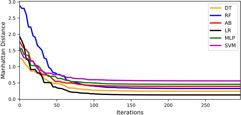
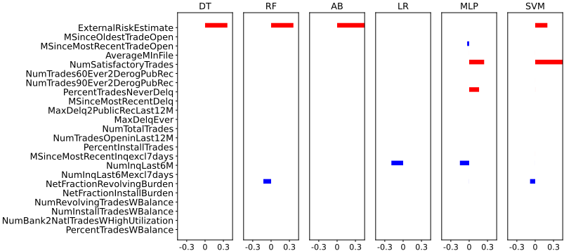
We also perform an extensive analysis of CMACE on a loan example of the Heloc dataset, which includes each individual's risk performance, credit score, load balance, history trade behavior, et al. We randomly select an individual instance with 23 credit risk features (all normalized), whose predictions are all negative (loan default) by six models (DT, RF, AB, LR, MLP, SVM) used in this work. In realistic situations, usually the counterfactual explanations are more actionable on condition that amount of features changed is smaller. So we consider the L1 norm as the distance function to compute the counterfactuals, on account of its regularization effect for perturbation sparsity. The minimization process of CMACE with different models is displayed in Figure 1, which shows that the convergence rate for searching optimal counterfactuals is fast, and the minimal distances of CFs to the original feature instance with different models are different. Figure 2 presents six results of counterfactual perturbations corresponding to different models, representative of six different ways to change personal risk features in order to get the loan.
From Figure 2, we observe that CFs of all the treebased models (DT, RF, AB) suggest that increasing ExternalRiskEstimate contributes to reduce the forecasting default probabilities and get approval by these models despite the increase amplitude is different, which indicates that the tree-based models treat ExternalRiskEstimate as the most important feature of this individual. The definitions of 23 features are available in the data dictionary. ExternalRiskEstimate belongs to a kind of credit score, so the counterfactual results conform to the feature definition that a higher score corresponds to a lower probability for loan default. Besides increasing ExternalRiskEstimate, the RF explanation also suggest concurrently decreasing another feature (NetFractionRevolvingBurden), which is in accord with the case in the work of FOCUS. Since NetFractionRevolvingBurden is the revolving balance divided by credit limit, the decreasing suggestion satisfies the causal common knowledge. In the remaining non tree-based models, the SVM explanation also suggest increasing the credit score feature by a moderate amplitude, while NumSatisfactoryTrades is recommended to be increased with a greatest amplitude and NetFractionRevolvingBurden is to be decreased slightly. NumSatisfactoryTrades is the number of satisfactory credit trades, which is regarded as the most sensitive feature by the SVM explanation. A larger NumSatisfactoryTrades means that the default probability of an individual is lower. As types of LR and MLP are different from those of tree-based models, features perturbed by the corresponding CFs are also different, both of which suggest decreasing NumInqLast6M, the number of inquiries by the lenders in the past six months. The larger number of inquiries represents that the individual attempted to submit loan applications to more financing institutions such as banks, which usually indicates a higher probability of loan default. While the simple LR model perturbs only one feature, the MLP explanation also suggest synchronously increasing NumSatisfactoryTrades and PercentTradesNeverDelq, and slightly decreasing MSinceMostRecentT radeOpen. PercentTradesNeverDelq is the percentage of trades that have never been delinquent, that is to say, the larger the percentage, the better the individual. And MSinceMostRecentTradeOpen means the number of months that the credit account has never been opened, which determine an individual's credit worthiness. In general, the perturbed features are on the whole actionable, except for the credit score feature belonging to a sort of black-box feature. Even so, increasing an individual's credit score is also feasible, which needs to know how the credit score is modelled and is out of scope of this work. In summary, we discover that the counterfactuals generated by CMACE basically conform to the causal relation between the applicant' feature change and the probability of potential loan.
| Dataset | Metric | Method | LR | MLP | SVM |
|---|---|---|---|---|---|
| Heloc | dmean | BayCon CMACE | 0.349 0.113 | 0.424 0.246 | 0.494 0.422 |
| %closer #CFs | CMACE<BayCon BayCon | 99.7% 3,138 | 85.7% 3,138 | 56.0% 3,137 | |
| Wine | generated dmean | CMACE BayCon CMACE | 3,138 0.276 0.200 | 3,138 0.274 0.204 | 3,138 0.314 0.219 |
| %closer #CFs generated | CMACE<BayCon BayCon CMACE | 100% 1,467 1,470 | 89.9% 1,470 1,470 | 91.9% 1,453 1,470 | |
| Compas | dmean | BayCon CMACE | 0.151 0.123 | 0.132 0.110 | 0.126 0.106 |
| %closer | CMACE<BayCon | 100% | 96.7% | 98.9% | |
| #CFs generated | BayCon CMACE | 1,843 1,852 | 1,851 1,852 | 1,846 1,852 | |
| Shopping | dmean | BayCon CMACE | 0.266 0.064 | 0.079 0.010 | 0.114 0.068 |
| %closer | CMACE<BayCon | 100% | 99.9% | 99.9% | |
| #CFs generated | BayCon CMACE | 3,683 3,699 | 3,696 3,699 | 3,653 3,699 |
5 Discussion and Conclusion
We propose a highly effective model-agnostic counterfactual explanation approach, CMACE, which dedicates to deal with the trade-off dilemma between better performance of modelspecific approaches and better scalability of model-agnostic approaches. Extensive experimental results demonstrate that besides scalable to various types of models, CMACE can not only significantly outperform SOTA model-agnostic approaches, but also outperform SOTA model-specific approaches, in terms of fundamental metrics such as mean distance. Furthermore, while pursuing higher performance, CMACE can generate counterfactuals with high sparsity, that is an important consideration for practical applications, because it is easier to understand shorter explanations [Miller, 2019; Naumann and Ntoutsi, 2021] and take corresponding actions. Moreover, CMACE can also generate counterfactuals in accord with the causal common sense, that is also a desirable property for counterfactual explanations.
Lastly, we discuss the limitations of our approach. We note that CMACE may be not applicable to super high dimension problems of generating counterfactuals, especially for the complex situation that the dimension of features exceeds the order of 103 . Generally, the amount of effective features for tabular data is rarely greater than 102 , so curse of dimensionality is not a problem. However, when counterfactual explanation is applied to image data with innumerable pixels, the corresponding search space is so large that our approach may not find optimal counterfactual perturbations. To our knowledge, only gradient-based approaches can handle this kind of problem. Our next work plan is to explore the problem of counterfactuals generating for image data by combining both advantages of gradient-based approaches and our approach.
Acknowledgments
This work was supported by National Key RD Program of China (2022YFB4501500, 2022YFB4501504) and the Key RD Program of Zhejiang (2024C01036).
@inproceedings{ijcai2024p60,
  title     = {CMACE: CMAES-based Counterfactual Explanations for Black-box Models},
  author    = {Yin, Xudong and Yang, Yao},
  booktitle = {Proceedings of the Thirty-Third International Joint Conference on
               Artificial Intelligence, {IJCAI-24}},
  publisher = {International Joint Conferences on Artificial Intelligence Organization},
  editor    = {Kate Larson},
  pages     = {539--547},
  year      = {2024},
  month     = {8},
  note      = {Main Track},
  doi       = {10.24963/ijcai.2024/60},
  url       = {https://doi.org/10.24963/ijcai.2024/60},
}
TY - CPAPER TI - CMACE: CMAES-based Counterfactual Explanations for Black-box Models AU - Yin, Xudong AU - Yang, Yao T2 - Proceedings of the Thirty-Third International Joint Conference on Artificial Intelligence, IJCAI-24 PB - International Joint Conferences on Artificial Intelligence Organization PY - 2024 SP - 539 EP - 547 DO - 10.24963/ijcai.2024/60 UR - https://doi.org/10.24963/ijcai.2024/60 ER -Copied
Machine-readable versions of this paper, for tools and AI agents:





