
Learning Pareto Set for Multi-Objective Continuous Robot Control
Proceedings of the Thirty-Third International Joint Conference on Artificial Intelligence. Main Track. Pages 4920-4928.
https://doi.org/10.24963/ijcai.2024/544
Keywords
- Robotics: ROB: Learning in robotics
- Machine Learning: ML: Optimization
- Machine Learning: ML: Reinforcement learning
Abstract
For a control problem with multiple conflicting objectives, there exists a set of Pareto-optimal policies called the Pareto set instead of a single optimal policy. When a multi-objective control problem is continuous and complex, traditional multi-objective reinforcement learning (MORL) algorithms search for many Pareto-optimal deep policies to approximate the Pareto set, which is quite resource-consuming. In this paper, we propose a simple and resource-efficient MORL algorithm that learns a continuous representation of the Pareto set in a high-dimensional policy parameter space using a single hypernet. The learned hypernet can directly generate various well-trained policy networks for different user preferences. We compare our method with two state-of-the-art MORL algorithms on seven multi-objective continuous robot control problems. Experimental results show that our method achieves the best overall performance with the least training parameters. An interesting observation is that the Pareto set is well approximated by a curved line or surface in a high-dimensional parameter space. This observation will provide insight for researchers to design new MORL algorithms.
- [Abels et al., 2019] Axel Abels, Diederik Roijers, Tom Lenaerts, Ann Nowé, and Denis Steckelmacher. Dynamic weights in multi-objective deep reinforcement learning. In International Conference on Machine Learning, vol- ume 97, pages 11-20, Jun 2019.
- [Alegre et al., 2023] Lucas N. Alegre, Ana L. C. Bazzan, Diederik M. Roijers, Ann Nowé, and Bruno C. da Silva. Sample-efficient multi-objective learning via generalized policy improvement prioritization. In Autonomous Agents and Multi-Agent Systems, page 2003-2012, 2023.
- [Barreto et al., 2020] André Barreto, Shaobo Hou, Diana Borsa, David Silver, and Doina Precup. Fast reinforcement learning with generalized policy updates. In Proceedings of the National Academy of Sciences, 2020.
- [Basaklar et al., 2023] Toygun Basaklar, Suat Gumussoy, and Umit Ogras. PD-MORL: Preference-driven multi- objective reinforcement learning algorithm. In Interna- tional Conference on Learning Representations, 2023.
- [Beck et al., 2023] Jacob Beck, Matthew Thomas Jackson, Risto Vuorio, and Shimon Whiteson. Hypernetworks in meta-reinforcement learning. In Proceedings of The 6th Conference on Robot Learning, volume 205, pages 1478- 1487, 2023.
- [Chauhan et al., 2023] Vinod Kumar Chauhan, Jiandong Zhou, Ping Lu, Soheila Molaei, and David A Clifton. A brief review of hypernetworks in deep learning. arXiv preprint arXiv:2306.06955, 2023.
- [Chen et al., 2019] Xi Chen, Ali Ghadirzadeh, Mårten Björkman, and Patric Jensfelt. Meta-learning for multi- objective reinforcement learning. In IEEE/RSJ Inter- national Conference on Intelligent Robots and Systems (IROS), pages 977-983. IEEE, 2019.
- [Galanti and Wolf, 2020] Tomer Galanti and Lior Wolf. On the modularity of hypernetworks. In Advances in Neu- ral Information Processing Systems, volume 33, pages 10409-10419, 2020.
- [Hayes et al., 2022] Conor F. Hayes, Roxana Rȃdulescu, Eu- genio Bargiacchi, Johan Källström, Matthew Macfarlane, Mathieu Reymond, Timothy Verstraeten, Luisa M. Zint- graf, Richard Dazeley, Fredrik Heintz, et al. A practi- cal guide to multi-objective reinforcement learning and planning. Autonomous Agents and Multi-Agent Systems, 36(1):26, 2022.
- [Hillermeier, 2001] Claus Hillermeier. Nonlinear multiob- jective optimization: a generalized homotopy approach, volume 135. Springer Science & Business Media, 2001.
- [Huang et al., 2021] Yizhou Huang, Kevin Xie, Homanga Bharadhwaj, and Florian Shkurti. Continual model-based reinforcement learning with hypernetworks. In IEEE International Conference on Robotics and Automation (ICRA), pages 799-805, 2021.
- [Lin et al., 2019] Xi Lin, Hui-Ling Zhen, Zhenhua Li, Qing- Fu Zhang, and Sam Kwong. Pareto multi-task learning. In Advances in Neural Information Processing Systems, vol- ume 32, 2019.
- [Lin et al., 2022] Xi Lin, Zhiyuan Yang, and Qingfu Zhang. Pareto set learning for neural multi-objective combinato- rial optimization. In International Conference on Learning Representations, 2022.
- [Lu et al., 2023] Haoye Lu, Daniel Herman, and Yaoliang Yu. Multi-objective reinforcement learning: Convexity, stationarity and Pareto optimality. In International Con- ference on Learning Representations, 2023.
- [Navon et al., 2021] Aviv Navon, Aviv Shamsian, Ethan Fe- taya, and Gal Chechik. Learning the pareto front with hypernetworks. In International Conference on Learning Representations, 2021.
- [Owen and Zhou, 2000] Art Owen and Yi Zhou. Safe and effective importance sampling. Journal of the American Statistical Association, 95(449):135-143, 2000.
- [Parisi et al., 2014] Simone Parisi, Matteo Pirotta, Nicola Smacchia, Luca Bascetta, and Marcello Restelli. Policy gradient approaches for multi-objective sequential deci- sion making. In International Joint Conference on Neural Networks, pages 2323-2330, 2014.
- [Parisi et al., 2017] Simone Parisi, Matteo Pirotta, and Jan Peters. Manifold-based multi-objective policy search with sample reuse. Neurocomputing, 263:3-14, 2017.
- [Pirotta et al., 2015] Matteo Pirotta, Simone Parisi, and Mar- cello Restelli. Multi-objective reinforcement learning with continuous pareto frontier approximation. In Proceed- ings of the AAAI Conference on Artificial Intelligence, vol- ume 29, 2015.
- [Rame et al., 2023] Alexandre Rame, Guillaume Couairon, Corentin Dancette, Jean-Baptiste Gaya, Mustafa Shukor, Laure Soulier, and Matthieu Cord. Rewarded soups: to- wards pareto-optimal alignment by interpolating weights fine-tuned on diverse rewards. In Advances in Neural In- formation Processing Systems, 2023.
- [Rezaei-Shoshtari et al., 2023] Sahand Rezaei-Shoshtari, Charlotte Morissette, Francois R. Hogan, Gregory Dudek, and David Meger. Hypernetworks for zero-shot transfer in reinforcement learning. In Proceedings of the AAAI Conference on Artificial Intelligence, volume 37, pages 9579-9587, Jun. 2023.
- [Roijers et al., 2013] Diederik M Roijers, Peter Vamplew, Shimon Whiteson, and Richard Dazeley. A survey of multi-objective sequential decision-making. Journal of Ar- tificial Intelligence Research, 48:67-113, 2013.
- [Roijers et al., 2018] Diederik M Roijers, Denis Steckel- macher, and Ann Nowé. Multi-objective reinforcement learning for the expected utility of the return. In Pro- ceedings of the Adaptive and Learning Agents Workshop at FAIM, 2018.
- [Sarafian et al., 2021] Elad Sarafian, Shai Keynan, and Sarit Kraus. Recomposing the reinforcement learning build- ing blocks with hypernetworks. In International Con- ference on Machine Learning, volume 139, pages 9301- 9312, 2021.
- [Schulman et al., 2017] John Schulman, Filip Wolski, Pra- fulla Dhariwal, Alec Radford, and Oleg Klimov. Prox- imal policy optimization algorithms. arXiv preprint arXiv:1707.06347, 2017.
- [Shang et al., 2021] Ke Shang, Hisao Ishibuchi, Linjun He, and Lie Meng Pang. A survey on the hypervolume indi- cator in evolutionary multiobjective optimization. IEEE Transactions on Evolutionary Computation, 25(1):1-20, 2021.
- [Van der Maaten and Hinton, 2008] Laurens Van der Maaten and Geoffrey Hinton. Visualizing data using t-SNE. Jour- nal of Machine Learning Research, 9(11), 2008.
- [Van Moffaert and Nowé, 2014] Kristof Van Moffaert and Ann Nowé. Multi-objective reinforcement learning using sets of pareto dominating policies. Journal of Machine Learning Research, 15(1):3483-3512, 2014.
- [von Oswald et al., 2020] Johannes von Oswald, Christian Henning, Benjamin F. Grewe, and João Sacramento. Con- tinual learning with hypernetworks. In International Con- ference on Learning Representations, 2020.
- [Xu et al., 2020] Jie Xu, Yunsheng Tian, Pingchuan Ma, Daniela Rus, Shinjiro Sueda, and Wojciech Matusik. Prediction-guided multi-objective reinforcement learning for continuous robot control. In International Conference on Machine Learning, pages 10607-10616, 2020.
- [Yang et al., 2019] Runzhe Yang, Xingyuan Sun, and Karthik Narasimhan. A generalized algorithm for multi- objective reinforcement learning and policy adaptation. In Advances in Neural Information Processing Systems, vol- ume 32, 2019.
- [Zhang and Li, 2007] Qingfu Zhang and Hui Li. MOEA/D: A multiobjective evolutionary algorithm based on decom- position. IEEE Transactions on Evolutionary Computa- tion, 11(6):712-731, 2007.
- [Zitzler et al., 2003] Eckart Zitzler, Lothar Thiele, Marco Laumanns, Carlos M Fonseca, and Viviane Grunert Da Fonseca. Performance assessment of multiobjective optimizers: An analysis and review. IEEE Transactions on Evolutionary Computation, 7(2):117-132, 2003.
References were extracted automatically from the PDF and may contain errors.
Full text extracted automatically from the PDF; figures, tables and equations may differ. The PDF is the version of record.
1 Introduction
In many real-world control problems, we often have multiple conflicting objectives. For example, in walking robot control, we may need to maximize walking speed and minimize energy consumption. Instead of a single optimal control policy, such a multi-objective control problem has a set of Pareto-optimal control policies called the Pareto set. Each Pareto-optimal policy in the Pareto set corresponds to a different trade-off (i.e., a different user preference) over conflicting objectives. To find these Pareto-optimal policies, multi-objective reinforcement learning (MORL) algorithms are widely used [Roijers et al., 2013; Hayes et al., 2022; Rame et al., 2023].
*Corresponding authors.
Many MORL algorithms [Van Moffaert and Now´e, 2014; Parisi et al., 2014; Xu et al., 2020] search for a finite set of independent policies to approximate the Pareto set. These algorithms have two potential drawbacks when handling continuous multi-objective control problems. One drawback is that a finite number of policies cannot represent the entire Pareto set. Thus, the following undesirable situation can happen: No policy in the obtained finite policy set is close to the user preference. The other drawback is that these methods are memory-consuming when the control problem has many objectives. This is because the number of required policies to approximate the Pareto set increases exponentially as the number of objectives increases. For example, more than 1,000 Pareto-optimal deep policies (represented by deep neural networks) are stored by an evolutionary learning algorithm for a three-objective robot control problem [Xu et al., 2020].
One idea to address these drawbacks is to train a single deep neural network to represent the whole Pareto set [Pirotta et al., 2015; Yang et al., 2019; Basaklar et al., 2023]. Based on this idea, two different types of methods have been proposed: embedding-based method and manifoldbased method. The embedding-based methods learn a generalized policy whose output is conditioned on the input preference [Yang et al., 2019; Abels et al., 2019; Basaklar et al., 2023]. These algorithms are usually off-policy algorithms with a specifically designed experience replay strategy. The Bellman equation is extended into a multi-objective version by including the user preference [Yang et al., 2019; Basaklar et al., 2023]. To improve the sample efficiency, Alegre et al. [2023] proposed a novel preference selection strategy based on Generalized Policy Improvement (GPI) [Barreto et al., 2020]. The manifold-based methods learn a parametric function to directly approximate the Pareto set as a manifold in the policy parameter space. For example, Pirotta et al. [2015] proposed a gradient-based approach called PMGA. Parisi et al. [2017] improved PMGA by using the importance sampling technique [Owen and Zhou, 2000]. However, these manifold-based approaches have not yet been applied to deep policies with tens of thousands of parameters. Two difficulties have been pointed out for these manifold-based methods in the literature: (1) The number of required parameters to represent the Pareto set is much more than (e.g., quadratically increases with) the dimensionality of the parameter space [Chen et al., 2019; Basaklar et al., 2023], and (2) the Pareto set in the parameter space cannot be efficiently represented by a single continuous policy family [Xu et al., 2020].
In this paper, we propose a manifold-based approach called Hyper-MORL to learn the Pareto sets (i.e., to search for Pareto-optimal deep policies) of multi-objective continuous control problems. Our assumption is that the Pareto set in a high-dimensional parameter space could be well approximated by a continuous manifold in a low-dimensional subspace. This assumption comes from the following property of multi-objective optimization: In general, the Pareto set of an m-objective problem is an (m - 1)-dimensional manifold in an n-dimensional parameter space even if n ≫ m [Hillermeier, 2001]. Based on this assumption, we propose an onpolicy MORL algorithm to learn a hypernet that maps a user preference (represented by a direction vector) to a Paretooptimal policy (represented by a point) in the parameter subspace. We examine our method on several complex multiobjective robot control problems [Xu et al., 2020] which are usually solved by deep policies with tens of thousands of parameters. Compared with two state-of-the-art MORL algorithms [Xu et al., 2020; Basaklar et al., 2023], our method shows the best overall performance with the least training parameters. To validate our initial assumption, we investigate the Pareto set learned by our method. We show that the Pareto set of continuous robot control problems can be well approximated by a single continuous policy family.
2 Background
2.1 Multi-Objective Markov Decision Process
A multi-objective RL problem (e.g., multi-objective continuous robot control problem) is usually modeled as a multi-objective Markov decision process (MOMDP). An MOMDP is described by the tuple ⟨S,A, P,R, γ⟩ where S, A, P(s′ |s, a), R and γ represent state space, action space, probability transition function, reward function and discount factor, respectively. Here the reward function R: S ×A → Rm returns a reward vector r = (r1, r2, ..., rm) where m is the number of objectives.
For an MOMDP, a policy π(a|s) represents the probability of selecting the action a ∈ A at the state s ∈ S. In each time step t, an agent with the policy π receives a state s(t) and selects an action a(t) ∼ π(a|s(t) ). Then, a reward vector r(t+1) = R(s(t) , a(t) ) and the next state s(t+1) ∼ P(s|s(t) , a(t) ) are given by the MOMDP. In this manner, we can obtain a trajectory τ = (s(0) , a(0) , r(1) , ..., s(T-1) , a(T-1) , r(T) ) where s(0) is the initial state and T is the time horizon. The expected returns J(π) = (J1(π), J2(π), ..., Jm(π)) is defined as:
where r(t) i is the i-th component of the reward vector r(t) .
Our target is to find a set of Pareto-optimal policies (called Pareto set) to maximize J. Here the optimality is defined by the Pareto dominance relation as follows.
Definition1 (Pareto Dominance Relation). A policy π is said to be dominated by another policy π′ (i.e., π′ ≻ π) iff ∀i ∈
In this paper, we assume a policy π(a|s, θ) (πθ for short) is parameterized by θ ∈ Θ ⊆ Rn where Θ is the parameter space. The Pareto set PS(Θ) in the parameter space is defined as
The image of PS(Θ) in the objective space is Pareto front.
2.2 Hypernets
Hypernets are a type of neural networks that take a context vector as input and generate the parameters for the target neural networks [Chauhan et al., 2023]. Compared with traditional neural networks, hypernets can be trained in a singlemodel manner to generate weights for multiple neural networks for solving related tasks [von Oswald et al., 2020]. Due to its parameter-efficiency and expressiveness [Galanti and Wolf, 2020], hypernets have been used in many fields such as reinforcement learning [Sarafian et al., 2021]. A taskconditioned hypernet is used for generalization across tasks in meta-RL [Beck et al., 2023]. Besides, hypernets have been used in continual RL [Huang et al., 2021] and zero-shot learning [Rezaei-Shoshtari et al., 2023] in RL.
Recently, hypernets have been used to learn the Pareto set for many multi-objective problems such as multi-objective combinatorial optimization [Lin et al., 2022] and multi-task learning [Navon et al., 2021; Lin et al., 2019]. In this paper, we use a hypernet to learn the Pareto set PS(Θ) of an MOMDP.
3 ProposedMethod: Hyper-MORL
To solve a multi-objective RL problem, we propose an efficient manifold-based algorithm called Hyper-MORL.
3.1 ProblemDecomposition
For multi-objective optimization, decomposition is a commonly-used idea [Zhang and Li, 2007]. A multiobjective RL (MORL) problem can be decomposed into several single-objective subproblems using a preference set {ω(1) ,ω(2) , ...,ω(k) } and a scalarization function f. Each subproblem with preference ω is a single-objective RL problem SORL(ω) which aims to maximize a scalar expected return f (J , ω).
The scalarization function f has two types: linear and nonlinear. The linear scalarization function fLS(J,ω) = ωT J is straightforward and widely used in many MORL algorithms [Parisi et al., 2014; Xu et al., 2020]. However, one limitation of fLS is that it can only find a convex hull, which is a subset of the Pareto set [Hayes et al., 2022]. Non-linear scalarization functions can find the whole Pareto set regardless of the Pareto front shape. However, the use of non-linear scalarization functions in RL is difficult since the assumed additive property in the Bellman equation does not hold for the non-linearly scalarized returns [Roijers et al., 2018; Hayes et al., 2022].
In this paper, we consider the linear scalarization function since Lu et al. [2023] theoretically revealed that a MORL
problem is convex (i.e., the range of the value function is convex) when all stationary policies are considered. Given a preference space Ω = {ω|ω ∈ ({0} ∪R+)m, ∑mi=1 ωi = 1}, the following proposition holds.
Proposition1 [Lu et al., 2023]. For a convex MORL problem, a policy π ∈ PS(Θ) iff ∃ω ∈ Ω, π is optimal for the problem SORL(ω) which maximizes ωT J(π).
Proposition 1 says that we can find the whole Pareto set by solving the problem SORL(ω) for each preference ω ∈ Ω.
3.2 Pareto Set Representation via Hypernet
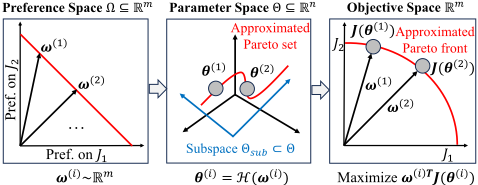
The basic idea of Hyper-MORL is shown in Figure 1. To represent the Pareto set, we train a model to map each preference ω ∈ Ω to the corresponding Pareto-optimal policy parameter θ ∈ Θ which maximizes ωT J(θ). To reduce the number of the required parameters, we consider a reduced d-dimensional subspace Θsub instead of the original n-dimensional parameter space Θ to represent the Pareto set (d ≪ n). The value of d is specified as 10 in this paper (and some other values are also examined for sensitivity analysis). A hypernet Hφ: Ω → Θ is defined as:
Here fµ maps the preference ω to a d-dimensional vector. The parameters W and b are an n × d matrix and an ndimensional vector, respectively. The row vectors of W spans a d-dimensional parameter subspace Θsub. The vector fµ(ω) is linearly transformed from Θsub to Θ. The learning parameters φ of the hypernet Hφ are {W, µ, b}. A detailed illustration of Hφ is included in Appendix 1 B.
3.3 Pareto Set Learning via Policy Gradient
To efficiently learn the Pareto set, a gradient-based algorithm is proposed for Hyper-MORL. As shown in Algorithm 1, the learning algorithm contains warm-up stage and Pareto set learning stage. As shown in lines 1-2, α×100% computation load is assigned to the warm-up stage where α is a parameter. In the following part, we will describe these two stages.
1 https://github.com/HisaoLabSUSTC/Hyper-MORL/blob/ main/Appendix.pdf
Algorithm 1: Learning Pareto Set via Policy Gradient
Input: Hypernet Hφ: Ω → Θ with parameters φ = {W, µ, b}, the number of sampled preferences K, the number of available environment steps T , parameter α 1 GW = ⌊ αT Ttra ⌋; 2 GPSL = ⌊ (1-α)T KTtra ⌋; // Ttra is the number of consumed environment steps to collect a trajectory 3 // Warm-up Stage 4 W ← 0; 5 Set µ and b by an arbitrary initialization scheme; 6 ω = ( 1m , ..., 1m ); 7 for g ← 1 to GW do 8 Run policy πb in environment and collect a trajectory τ ; 9 Calculate gradients g ←∇b[ωT J(b)]; 10 Update parameters b ←ADAM(b, g); 11 Reset exploration-related parameters in b; 12 // Pareto Set Learning Stage 13 for g ← 1 to GPSL do 14 Sample K preferences ω(1) , ..., ω(K) fromΩ; 15 for i ← 1 to K do 16 Run policy πHφ(ω(i) ) in environment and collect a trajectory τ (i) ; 17 for i ← 1 to K do 18 Calculate gradients g(i) ← ∇φ[ω(i)T J(Hφ(ω(i) ))] 19 Update parameters φ←ADAM(φ, 1K ∑Ki=1 g(i) );Warm-up Stage
The warm-up stage is to find a good initial policy close to the Pareto front. By starting from a good initial policy instead of a random policy, the Pareto set learning stage can be accelerated. In Algorithm 1, the warm-up stage is in lines 3-11. In lines 4-5, we use the Bias-HyperInit method [Beck et al., 2023] to initialize the hypernet parameters. In lines 6-10, we update parameters b to optimize all objectives simultaneously with the preference ( 1m , ..., 1m ) (m is the number of objectives). The multi-objective policy gradient method [Xu et al., 2020] is used as follows:
where A is the advantage function estimated from a sampled trajectory τ .
After GW iterations, we obtain a policy πb from the preference ( 1m , ..., 1m ). In our implementation, the policy πb samples an action from a normal distribution. Some values in the n-dimensional vector b represent the standard deviation of the output action. In line 11, the exploration-related parameters (i.e., the standard deviation of the output action) are reset as one. Since other values in b are not changed, the mean of the output action is preserved. The reset step is to prevent the output action selection from being almost deterministic (i.e., standard deviation from being almost zero) which severely degrades the exploration ability in the Pareto set learning stage. After the warm-up stage, b becomes closer to the Pareto set, and W remains 0. From Eq. (3), the hypernet Hφ(ω) = b for ∀ω ∈ Ω. This means that the initial values of b are shared among all subproblems.
Pareto Set Learning Stage
Our task is to find the optimal parameters φ (i.e., W, µ and b) which maximizes ωT J(Hφ(ω)) for each ω ∈ Ω. The objective function can be written as:
It is difficult to directly optimize the parameters φ to maximize the exception in Eq. (5). Thus, we use Monte Carlo method to sample the preferences, and use the policy gradient method to optimize the parameters φ. In Algorithm 1, lines 13-19 show the Pareto set learning stage. In each iteration, K preferences are randomly sampled from the preference space Ω. Then, we obtain K policies by inputting these K preferences into the hypernet. In lines 15-16, each policy interacts with the environment and generates a trajectory. In lines 17-18, the gradient g(i) is calculated for each preference based on the corresponding trajectory. Then, the parameters φ are updated based on the average gradient over all sampled preferences (i.e., 1K ∑Ki=1 g(i) ).
The remaining question is how to calculate the gradient g(i) in line 18. By the chain rule, we have
where θ = Hφ(ω) and · means dot product. As we can see, the term ∇θ [ωT J(θ)] can be calculated by Eq. (4). Thus, the gradient g(i) can be calculated by Eq. (4) and Eq. (6). After the Pareto set learning stage, the whole Pareto set PS(Θ) is obtained from the hypernet Hφ.
4 Experiments
4.1 Benchmark Problems
To test the performance of Hyper-MORL, we use seven problems in Table 1 from a multi-objective robot control benchmark suite [Xu et al., 2020]. For more details, please refer to Appendix A.
4.2 ComparedMORL Algorithms
We compare the proposed Hyper-MORL algorithm with the following two state-of-the-art MORL algorithms.
PG-MORL [Xu et al., 2020]
Prediction-guided MORL (i.e., PG-MORL) algorithm is an evolutionary learning algorithm. In each generation, PGMORL selects a set of policies from the current population based on a prediction model, and optimizes them with a multi-objective policy gradient method. All Pareto-optimal policies are stored in an unbounded external archive. We use the default settings in the original paper for PG-MORL 2 .
| Problem | m | State space | Action space |
|---|---|---|---|
| MO-Swimmer-v2 | 2 | S ⊆ R8 | A ⊆ R2 |
| MO-HalfCheetah-v2 | 2 | S ⊆ R17 | A ⊆ R6 |
| MO-Walker2d-v2 | 2 | S ⊆ R17 | A ⊆ R6 |
| MO-Ant-v2 | 2 | S ⊆ R27 | A ⊆ R8 |
| MO-Hopper-v2 | 2 | S ⊆ R11 | A ⊆ R3 |
| MO-Humanoid-v2 | 2 | S ⊆ R376 | A ⊆ R17 |
| MO-Hopper-v3 | 3 | S ⊆ R11 | A ⊆ R3 |
| Problem | Hyper-MORL | PG-MORL | PD-MORL |
|---|---|---|---|
| MO-Swimmer-v2 | 1.2×10⁷ | 1.2×10⁷ | 1 × 10⁷ |
| MO-Walker2d-v2 | 3 × 10⁷ | 3 × 10⁷ | 1 × 10⁷ |
| MO-HalfCheetah-v2 | 3 × 10⁷ | 3 × 10⁷ | 1 × 10⁷ |
| MO-Ant-v2 | 4.8×10⁷ | 4.8×10⁷ | 1 × 10⁷ |
| MO-Hopper-v2 | 4.8×10⁷ | 4.8×10⁷ | 1 × 10⁷ |
| MO-Humanoid-v2 | 1.2×10⁸ | 1.2×10⁸ | 1 × 10⁷ |
| MO-Hopper-v3 | 1.2×10⁸ | 1.2×10⁸ | 1 × 10⁷ |
PD-MORL [Basaklar et al., 2023]
Preference-driven MORL (i.e., PD-MORL) algorithm learns a generalized policy by combining the preference into the Bellman equation. We use the default settings in the original paper for PD-MORL 3 . Note that the number of environment steps used by PD-MORL is smaller than that used by PG-MORL as shown in Table 2. However, PD-MORL needs more computation time than PG-MORL, which we will discuss in Section 4.3. We find it impractical for PD-MORL to use the same number of environment steps as in PG-MORL.
Hyper-MORL (Our Algorithm)
In our algorithm, we use the same neural network architecture as in PG-MORL. Thus, the parameter spaces of HyperMORL and PG-MORL are the same. For a fair comparison, Hyper-MORL uses the same policy gradient method (i.e., PPO [Schulman et al., 2017]) as in PG-MORL. The optimizer is ADAM with learning rate η = 5 × 10⁻⁵ . In Hyper-MORL, the parameters α and d are set as 0.15 (i.e., 15%) and 10, respectively. The number of sampled preferences K is set as 6 and 15 for two-objective and threeobjective problems, respectively. For more details, please refer to Appendix C. All codes of Hyper-MORL are available from https://github.com/HisaoLabSUSTC/Hyper-MORL.
2 https://github.com/mit-gfx/PGMORL
| Algorithm | Hyper-MORL (Ours) | PG-MORL | PD-MORL |
|---|---|---|---|
| MO-Swimmer-v2 | 2.88±0.44 × 10⁴ (2) | 2.60±0.71 × 10⁴ (3) | 3.13±0.14×10⁴ (1) |
| MO-HalfCheetah-v2 | 5.53±0.10×10⁶ (3) | 5.75±0.02×10⁶ (2) | 5.89±0.01×10⁶ (1) |
| MO-Walker2d-v2 | 5.37±0.35×10⁶ (1) | 4.41±0.74×10⁶ (2) | 5.08±0.23×10⁶ (3) |
| MO-Ant-v2 | 7.49 ± 0.16 × 10⁶ (1) | 5.79±0.25×10⁶ (3) | 7.05±1.13×10⁶ (2) |
| MO-Hopper-v2 | 2.05 ± 0.06 × 10⁷ (1) | 1.96±0.17×10⁷ (2) | 5.84±8.12×10⁶ (3) |
| MO-Humanoid-v2 | 4.32±0.42×10⁷ (2) | 4.69±0.29×10⁷ (1) | 1.66±0.60×10⁷ (3) |
| MO-Hopper-v3 | 3.58±0.25×10¹⁰ (1) | 3.31±0.23×10¹⁰ (2) | 1.14±1.24×10¹⁰ (3) |
| Average Rank | 1.57 | 2.29 | 2.14 |
4.3 Performance Comparison
We first compare the quality of the policy sets learned by the three algorithms. A widely-used indicator hypervolume (HV) [Zitzler et al., 2003; Shang et al., 2021] is used for the quality assessment, which is explained in Appendix E. For the evolutionary learning algorithm (i.e., PG-MORL), we evaluate the final population with population sizes 200 and 420 for 2-objective and 3-objective problems, respectively. For a fair comparison, we sample the same number of uniformly distributed preferences for each of the single model-based algorithms (i.e., PD-MORL and Hyper-MORL), and evaluate the output policies. Table 3 shows the HV results of each algorithm on the seven test problems. As we can see, HyperMORL has the best HV performance on 4 out of 7 problems and the worst only on MO-HalfCheetah-v2. Thus, HyperMORL has the best average rank in Table 3.
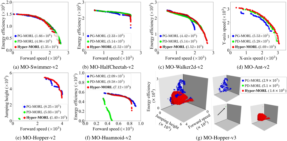
To test the ability of each algorithm to generate the continuous Pareto front, we use a single run with the median HV value for each algorithm. For PG-MORL, we plot all Paretooptimal policies stored in the unbounded external archive. For Hyper-MORL and PD-MORL, we input a number of uniform preferences and plot all Pareto-optimal policies corresponding to these preferences. The number of input preferences is set as 2,000 and 200,100 for 2-objective and 3objective problems, respectively. Figure 2 shows all Paretooptimal policies from each algorithm on each test problem. Except for MO-HalfCheetah-v2, Hyper-MORL generates a continuous approximation of the Pareto front with high quality for each problem. Especially for MO-Hopper-v3 in Figure 2 (g), Hyper-MORL generates a much more dense approximation than the other two methods. As shown in parenthesis in Figure 2, Hyper-MORL has the smallest number of parameters for each problem among three algorithms.
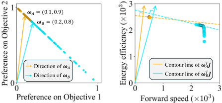
Hyper-MORL shows poor performance only on MOHalfCheetah-v2 in Figure 2 (b). The reason is explained in Figure 3. As we can see, many preferences are mapped to the top left corner of the objective space by Hyper-MORL. This is because the linear scalarization function cannot find solutions on flat and concave regions of the Pareto front. The search for those regions by non-linear scalarization function is a future research topic.
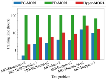
From Table 3 and Figure 2, we can see that PD-MORL (green points in Figure 2) has poor performance on MOHopper-v2, MO-Humanoid-v2, and MO-Hopper-v3, which could be due to two reasons. One reason is that the performance of PD-MORL highly relies on an interpolation procedure with some key solutions, as mentioned in the original paper [Basaklar et al., 2023]. However, PD-MORL could not find any good key solutions for these problems. The other reason is that the number of environment steps (shown in Table 2) in PD-MORL may be insufficient. Figure 4 shows the training time of each algorithm. As we can see, PD-MORL needs the longest training time. For MO-Humanoid-v2, the training in PD-MORL for 1 × 10⁷ environment steps needs about four days, while the training in Hyper-MORL and PGMORL for 1.2 × 10⁸ environment steps needs less than one day. If we use the same number of environment steps in all three algorithms, the training in PD-MORL will take about 40 days.
5 Further Studies
5.1 Investigation of the Learned Pareto Set
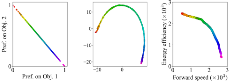
We further investigate the relation between the input preferences and the Pareto sets learned by Hyper-MORL. For better visualization, each preference is plotted with a different color in Figure 5 (a). Then, each policy in the learned Pareto set is plotted with the same color as its corresponding input preference in Figure 5 (b) and (c) for MO-Walker2d-v2. Dominated
- (a) Preference space (b) Parameter space (c) Objective space
Figure 5: Visualization of the Pareto-optimal policies obtained by Hyper-MORL for MO-Walker2d-v2 problem in the parameter space (b) and objective space (c), and their corresponding input to the hypernet in the preference space (a). Each policy is plotted with the same color as its corresponding input preference. t-SNE is used for visualization in the 11,150-dimensional parameter space.
policies and the related preferences are not shown in Figure 5. We show the learned Pareto set in both the parameter space and the objective space. Since the dimension of the parameter space is high, we use t-SNE [Van der Maaten and Hinton, 2008] to visualize the high-dimensional parameter space in a two-dimensional space. Visualization results for the other problems are included in Appendix D.1. In Figure 5, we can observe a clear relation between the preferences in (a) and the Pareto front in (c). For example, the top-left solution in Figure 5 (c) with the largest second objective value is obtained from the preference (0, 1).
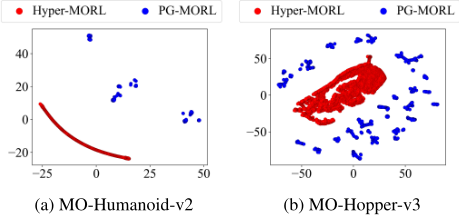
One interesting observation from Figure 5 (b) is that the shape of the Pareto set learned by Hyper-MORL is a simple curve after the dimensionality reduction from the 11,150dimensional parameter space. This observation is different from reported results on PG-MORL [Xu et al., 2020] where it was shown that a single continuous policy family cannot represent the Pareto set of these continuous robot control problems well. Thus, we further compare the two policy sets learned by Hyper-MORL and PG-MORL in the parameter space. PD-MORL is not considered since it has a different parameter space from Hyper-MORL and PG-MORL. Figure 6 shows the comparison results on the two-objective MOHumanoid-v2 and three-objective MO-Hopper-v3 problems. As we can see, Hyper-MORL learns a single continuous policy family in Figure 6 (a) and closely related policy families in Figure 6 (b) while PG-MORL learns a set of disjoint policy families.
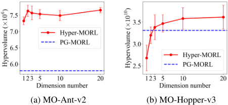
As discussed in Section 3.2, the Pareto set learned by Hyper-MORL is located in a d-dimensional parameter subspace where d is a parameter for the hypernet used in HyperMORL. We examine the effects of d on the hypervolume performance of Hyper-MORL using six values of d: d =1, 2, 3, 5, 10, 20. Figure 7 shows the results of the two-objective MO-Ant-v2 and three-objective MO-Hopper-v3 problems. As a baseline, the hypervolume performance of PG-MORL is shown by the blue dotted line. In Figure 7 (a), the hypervolume performance of Hyper-MORL is better than PGMORL even when d = 1. That means the Pareto set of MO-Ant-v2 is well approximated by Hyper-MORL with a curved line in the parameter space. For the three-objective MO-Hopper-v3 problem in Figure 7 (b), good results are obtained when d > 2. The results for the other problems are included in Appendix D.2. Our experimental results show that the Pareto sets of most problems are well approximated by Hyper-MORL in low-dimensional parameter subspace.
5.2 Effects of theWarm-Up Stage
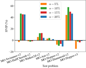
To examine the effects of the warm-up stage, we test four specifications of α: 0%, 5%, 10%, and 20%. α = 0% means that the warm-up stage is not performed, and the hypernet is initialized by the Bias-HyperInit [Beck et al., 2023]. All the other settings except for α are the same as in the previous experiments. For each specification (i.e., α = x%), we calculate the hypervolume improvement percentage (HVIP) from the results with α = 0% as follows:
Here positive and negative HVIP values mean positive and negative effects of the warm-up stage with α = x%. The HVIP results are shown in Figure 8. We can see that the warm-up stage has a large positive effect on the hypervolume performance for MO-Swimmer and MO-Humanoid-v2 (i.e., more than 40% improvement). For the other problems, the positive and negative effects of the warm-up stage are small (less than 10%). Figure 8 also shows that too small value (e.g., 5%) or too large value (e.g., 20%) for the parameter α is not good. Our recommended value for α is 15%.
6 Conclusions
In this paper, we proposed an MORL algorithm called HyperMORL, which learns a hypernet to approximate the Pareto set in a high-dimensional parameter space of deep policies by using a low-dimensional reduced parameter space. We compared Hyper-MORL with two state-of-the-art algorithms on seven multi-objective robot control problems. Our results showed that Hyper-MORL has the best overall performance and the least training parameters among compared algorithms. By the investigation of the Pareto set learned by Hyper-MORL, we found that the Pareto set of these multiobjective objective robot control problems can be well approximated by a manifold in a low-dimensional (e.g., 3dimensional) subspace of the original high-dimensional (e.g., 11,150-dimensional) parameter space. Our results provide valuable insights for researchers to design new MORL algorithms. In the future, we try to combine a non-linear scalarization function into our method.
Acknowledgments
This work was supported by National Natural Science Foundation of China (Grant No. 62250710163, 62376115), Guangdong Provincial Key Laboratory (Grant No. 2020B121201001).
@inproceedings{ijcai2024p544,
  title     = {Learning Pareto Set for Multi-Objective Continuous Robot Control},
  author    = {Shu, Tianye and Shang, Ke and Gong, Cheng and Nan, Yang and Ishibuchi, Hisao},
  booktitle = {Proceedings of the Thirty-Third International Joint Conference on
               Artificial Intelligence, {IJCAI-24}},
  publisher = {International Joint Conferences on Artificial Intelligence Organization},
  editor    = {Kate Larson},
  pages     = {4920--4928},
  year      = {2024},
  month     = {8},
  note      = {Main Track},
  doi       = {10.24963/ijcai.2024/544},
  url       = {https://doi.org/10.24963/ijcai.2024/544},
}
TY - CPAPER TI - Learning Pareto Set for Multi-Objective Continuous Robot Control AU - Shu, Tianye AU - Shang, Ke AU - Gong, Cheng AU - Nan, Yang AU - Ishibuchi, Hisao T2 - Proceedings of the Thirty-Third International Joint Conference on Artificial Intelligence, IJCAI-24 PB - International Joint Conferences on Artificial Intelligence Organization PY - 2024 SP - 4920 EP - 4928 DO - 10.24963/ijcai.2024/544 UR - https://doi.org/10.24963/ijcai.2024/544 ER -Copied
Machine-readable versions of this paper, for tools and AI agents:





