
Toward a Manifold-Preserving Temporal Graph Network in Hyperbolic Space
Proceedings of the Thirty-Third International Joint Conference on Artificial Intelligence. Main Track. Pages 4380-4388.
https://doi.org/10.24963/ijcai.2024/484
Keywords
- Machine Learning: ML: Geometric learning
- Machine Learning: ML: Sequence and graph learning
- Data Mining: DM: Mining spatial and/or temporal data
- Data Mining: DM: Mining graphs
Abstract
Hyperbolic geometry provides an ideal setting to represent the scale-free or hierarchical characteristics of an input graph naturally. Utilizing hyperbolic geometry for learning dynamic graph representation has gained a growing interest in recent years. However, the majority of hyperbolic-based approaches rely on tangent spaces to perform graph operations, which could distort the structure of the dynamic graph when the graph grows over time. To avoid the distortion in tangent space, we propose a Hyperbolic Manifold-Preserving Temporal Graph Network that works directly on the hyperbolic manifold. The model includes a graph convolution module for learning the spatial dependencies, an attention architecture for capturing the temporal properties, and a gated recurrent unit for extracting the spatio-temporal relationships. By evaluating on diverse real-world dynamic graphs, our model has achieved significant improvements in link prediction and new link prediction tasks, in comparison with other baselines.
- [Bai et al., 2023] Qijie Bai, Chang Nie, Haiwei Zhang, Dongming Zhao, and Xiaojie Yuan. Hgwavenet: A hyper- bolic graph neural network for temporal link prediction. Proceedings of the ACM Web Conference 2023, 2023.
- [Bjørnstad et al., 2002] Ottar N. Bjørnstad, Bärbel Finkenstädt, and Bryan T. Grenfell. Dynamics of measles epidemics: Estimating scaling of transmis- sion rates using a time series sir model. Ecological Monographs, 72:169-184, 2002.
- [Bronstein et al., 2017] Michael M. Bronstein, Joan Bruna, Yann LeCun, Arthur Szlam, and Pierre Vandergheynst. Geometric deep learning: Going beyond euclidean data. IEEE Signal Processing Magazine, 34(4):18-42, 2017.
- [Chami et al., 2019] Ines Chami, Rex Ying, Christopher Ré, and Jure Leskovec. Hyperbolic graph convolutional neu- ral networks. Advances in neural information processing systems, 32:4869-4880, 2019.
- [Chen et al., 2021a] Weize Chen, Xu Han, Yankai Lin, Hexu Zhao, Zhiyuan Liu, Peng Li, Maosong Sun, and Jie Zhou. Fully hyperbolic neural networks. ArXiv, abs/2105.14686, 2021.
- [Chen et al., 2021b] Yankai Chen, Menglin Yang, Yingxue Zhang, Mengchen Zhao, Ziqiao Meng, Jianye Hao, and Ir- win King. Modeling scale-free graphs with hyperbolic ge- ometry for knowledge-aware recommendation. Proceed- ings of the Fifteenth ACM International Conference on Web Search and Data Mining, 2021.
- [Cho et al., 2014] Kyunghyun Cho, Bart van Merrienboer, C ¸aglar Gülc ¸ehre, Fethi Bougares, Holger Schwenk, and Yoshua Bengio. Learning phrase representations using RNN encoder-decoder for statistical machine translation. CoRR, abs/1406.1078, 2014.
- [Dai et al., 2021] Jindou Dai, Yuwei Wu, Zhi Gao, and Yunde Jia. A hyperbolic-to-hyperbolic graph convolu- tional network. 2021 IEEE/CVF Conference on Computer Vision and Pattern Recognition (CVPR), pages 154-163, 2021.
- [Hajiramezanali et al., 2020] Ehsan Hajiramezanali, Arman Hasanzadeh, Nick Duffield, Krishna R Narayanan, Mingyuan Zhou, and Xiaoning Qian. Variational graph recurrent neural networks, 2020.
- [Kipf and Welling, 2016a] Thomas N. Kipf and Max Welling. Semi-supervised classification with graph convolutional networks. CoRR, abs/1609.02907, 2016.
- [Kipf and Welling, 2016b] Thomas N. Kipf and Max Welling. Variational graph auto-encoders, 2016.
- [Klimt and Yang, 2004] Bryan Klimt and Yiming Yang. In- troducing the enron corpus. In International Conference on Email and Anti-Spam, 2004.
- [Krioukov et al., 2010] Dmitri Krioukov, Fragkiskos Pa- padopoulos, Maksim Kitsak, Amin Vahdat, and Mariá n Boguñá. Hyperbolic geometry of complex networks. Physical Review E, 82(3), sep 2010.
- [Leskovec et al., 2007] Jure Leskovec, Jon Kleinberg, and Christos Faloutsos. Graph evolution: Densification and shrinking diameters, 2007.
- [Lezcano-Casado, 2019] Mario Lezcano-Casado. Trivial- izations for gradient-based optimization on manifolds. In Advances in Neural Information Processing Systems, NeurIPS, pages 9154-9164, 2019.
- [Li et al., 2023] Hao Li, Hao Jiang, Dongsheng Ye, Qiang Wang, Liang Du, Yuanyuan Zeng, Liu yuan, Yingxue Wang, and Cheng Chen. Dhgat: Hyperbolic representa- tion learning on dynamic graphs via attention networks. Neurocomputing, 2023.
- [Lin et al., 2023] Ya-Wei Eileen Lin, Ronald R. Coifman, Gal Mishne, and Ronen Talmon. Hyperbolic diffusion em- bedding and distance for hierarchical representation learn- ing. ArXiv, abs/2305.18962, 2023.
- [Liu et al., 2019] Qi Liu, Maximilian Nickel, and Douwe Kiela. Hyperbolic graph neural networks. ArXiv, abs/1910.12892, 2019.
- [Nguyen et al., 2018] Giang Hoang Nguyen, John Boaz Lee, Ryan A. Rossi, Nesreen Ahmed, Eunyee Koh, and Sungchul Kim. Continuous-time dynamic network em- beddings. Companion Proceedings of the The Web Con- ference 2018, 2018.
- [Panzarasa et al., 2009] Pietro Panzarasa, Tore Opsahl, and Kathleen M. Carley. Patterns and dynamics of users' be- havior and interaction: Network analysis of an online com- munity. J. Assoc. Inf. Sci. Technol., 60:911-932, 2009.
- [Paranjape et al., 2016] Ashwin Paranjape, Austin R. Ben- son, and Jure Leskovec. Motifs in temporal networks. Proceedings of the Tenth ACM International Conference on Web Search and Data Mining, 2016.
- [Pareja et al., 2019] Aldo Pareja, Giacomo Domeniconi, Jie Chen, Tengfei Ma, Toyotaro Suzumura, Hiroki Kanezashi, Tim Kaler, and Charles E. Leiserson. Evolvegcn: Evolving graph convolutional networks for dynamic graphs. CoRR, abs/1902.10191, 2019.
- [Peng et al., 2021] Wei Peng, Tuomas Varanka, Abdelrah- man Mostafa, Henglin Shi, and Guoying Zhao. Hyper- bolic deep neural networks: A survey. IEEE Transactions on Pattern Analysis and Machine Intelligence, 44:10023- 10044, 2021.
- [Rossi et al., 2013] Ryan A. Rossi, Brian Gallagher, Jennifer Neville, and Keith W. Henderson. Modeling dynamic be- havior in large evolving graphs. Proceedings of the sixth ACM international conference on Web search and data mining, 2013.
- [Rossi et al., 2020] Emanuele Rossi, Ben Chamberlain, Fab- rizio Frasca, Davide Eynard, Federico Monti, and Michael Bronstein. Temporal graph networks for deep learning on dynamic graphs. arXiv preprint arXiv:2006.10637, 2020.
- [Sankar et al., 2018] Aravind Sankar, Yanhong Wu, Liang Gou, Wei Zhang, and Hao Yang. Dynamic graph rep- resentation learning via self-attention networks. CoRR, abs/1812.09430, 2018.
- [Tuzel et al., 2008] Oncel Tuzel, Fatih Murat Porikli, and Peter Meer. Pedestrian detection via classification on rie- mannian manifolds. IEEE Transactions on Pattern Analy- sis and Machine Intelligence, 30:1713-1727, 2008.
- [Ungar, 2000] Abraham Ungar. Hyperbolic trigonometry and its application in the poincaré ball model of hyperbolic geometry. Computers & Mathematics with Applications, 41:135-147, 04 2000.
- [Ungar, 2005] Abraham A Ungar. Analytic hyperbolic geom- etry: Mathematical foundations and applications. World Scientific, 2005.
- [Weber et al., 2019] Mark Weber, Giacomo Domeniconi, Jie Chen, Daniel Karl I. Weidele, Claudio Bellei, Tom Robin- son, and Charles E. Leiserson. Anti-money laundering in bitcoin: Experimenting with graph convolutional networks for financial forensics, 2019.
- [Xue et al., 2021] Guotong Xue, Ming Zhong, Jianxin Li, Jia Chen, Chengshuai Zhai, and Ruochen Kong. Dynamic net- work embedding survey. CoRR, abs/2103.15447, 2021.
- [Yang and Leskovec, 2012] Jaewon Yang and Jure Leskovec. Defining and evaluating network commu- nities based on ground-truth. CoRR, abs/1205.6233, 2012.
- [Yang et al., 2021] Menglin Yang, Min Zhou, Marcus Ka- lander, Zengfeng Huang, and Irwin King. Discrete- time temporal network embedding via implicit hierarchi- cal learning in hyperbolic space. Proceedings of the 27th ACM SIGKDD Conference on Knowledge Discovery & Data Mining, 2021.
- [Yang et al., 2023] Menglin Yang, Min Zhou, Rex Ying, Yankai Chen, and Irwin King. Hyperbolic represen- tation learning: Revisiting and advancing. ArXiv, abs/2306.09118, 2023.
References were extracted automatically from the PDF and may contain errors.
Full text extracted automatically from the PDF; figures, tables and equations may differ. The PDF is the version of record.
1 Introduction
Many real-world complex networks [Leskovec et al., 2007; Weber et al., 2019] can be modeled as dynamic graphs. Learning representation of dynamic graph is a challenging but vital step to understand how the network interacts and evolves over time [Yang et al., 2021]. Dynamic graphs, based on how the graphs undergo updates, can be categorized into two groups: continuous-time dynamic graphs [Rossi et al., 2020] and discrete-time dynamic graphs [Xue et al., 2021].
In a discrete-time dynamic graph, the changes in the graph presumably occur at separate time points and the graph structure at each time point is called a snapshot. Researchers have presented various methods for capturing the spatial and temporal dependencies of discrete dynamic graphs such as EvolveGCN [Pareja et al., 2019] and VGRNN [Hajiramezanali et al., 2020]. These two methods use the graph recurrent framework by incorporating a graph neural network, e.g., GCN [Kipf and Welling, 2016a] and a gate recurrent unit, e.g., GRU [Cho et al., 2014] to learn the embedding of a dynamic graph. Most of the discrete-based approaches are designed to work on the well-known Euclidean space. Alternatively, [Bronstein et al., 2017] prove that many real-world graphs exhibit hierarchical structures and power-law distributions rather than uniform grid structures that best fit Euclidean space. In contrast to Euclidean geometry, hyperbolic geometry such as the Poincar´e ball model or the Lorentz model, is more suitable for embedding scale-free and hierarchical graphs because of its exponential expansion property [Krioukov et al., 2010].
∗Corresponding author: Viet Cuong Ta
Given the expressiveness of hyperbolic space in learning graph embedding, there has been an increasing interest in utilizing hyperbolic properties for learning representation of dynamic graph [Yang et al., 2021; Li et al., 2023]. Although hyperbolic methods have achieved state-of-the-art performance, their reliance on tangent space for graph operations is considered suboptimal. While the induced distance among two neighbor nodes' embedding on the hyperbolic manifold exhibits the hierarchical characteristic of the graph, it is not preserved after the mapping to the tangent space [Tuzel et al., 2008]. In other words, the distance in tangent space is only a first-order approximation of the induced distance, which results in a distortion of the hierarchical structure of the given graph [Krioukov et al., 2010; Lin et al., 2023]. To address this issue, [Dai et al., 2021] propose the H2H-GCN architecture which uses only the Lorentz model for graph operations, thus can avoid the distortion caused by projecting to tangent space. With the same purpose as H2H-GCN, DHGAT [Li et al., 2023] designs spatiotemporal aggregate functions without depending on tangent space for representation learning in dynamic graphs.
In this work, we first give a detailed analysis of the distortion errors caused by the hyperbolic tangent space in representation learning for dynamic graphs. We show that the errors, which mainly come from the forward projection to tangent space and its reverse mapping, have lower bounds and increase as the graph evolves. Hence, to overcome the ineffectiveness of hyperbolic tangent space approaches, we propose a Hyperbolic Manifold-Preserving Temporal Graph Network (HMPTGN) that works directly on the hyperbolic manifold, rather than in tangent space. Our proposed model is centralized by a hyperbolic feature transformation which constrains the transformation matrix to be orthogonal to ensure the node representation resides on the manifold. The hyperbolic feature transformation is then added to the standard graph neural network and gated recurrent unit to form the hyperbolic manifold-preserving graph neural network (HMPGNN) and hyperbolic manifold-preserving gated recurrent unit (HMPGRU) in the model, respectively. The HMPGNN is employed to capture spatial dependencies between nodes within the hyperbolic space, while the HMPGRU is used to extract the spatio-temporal representation of dynamic graph. An additional temporal attention component with manifold-preserving property (HMPTA) is integrated into the HMPTGN to extract the time-based relationship within a fixed-length historical window. We evaluate the performance of our model on two tasks, temporal link prediction task and new link prediction task on real-world dynamic graphs. The results demonstrate that our HMPTGN achieves significant improvements in comparison with other baselines, especially in new link prediction task.
2 Preliminaries
2.1 ProblemDefinition
A discrete-time dynamic graph is a collection of independent and complete snapshots {G1, G2, ..., GT} sampled from a dynamic graph G, where T is the number of snapshots and Gt is a snapshot at timestamp t. Each snapshot Gt has a particular node set Vt and a corresponding adjacency matrix At. Similar to [Pareja et al., 2019; Yang et al., 2021], our work is based on the graph recurrent framework which is defined as:
where Xt are the initial features of the node set Vt and Ht-1 is the latest historical state, ϕ is a graph neural network which aggregates local features and learns the node representation, and ψ is a recurrent model for learning the spatio-temporal properties. Possible choices for ϕ and ψ are GCN [Kipf and Welling, 2016a] and GRU [Cho et al., 2014], respectively.
2.2 Hyperbolic Geometry in Graph Embedding
In general graph representation learning, the embedding Ht with Euclidean distance is used to characterize the graph structure. The extension of the learned embedding Ht to a hyperbolic space requires the definition of a Riemannian manifold (M, g), which is a differentiable manifold M equipped with a Riemannian metric tensor g. Specifically, a hyperbolic space is a smooth Riemannian manifold with a constant negative curvature. Our work is built upon the Poincar´e ball model due to its conformality and stability in learning graph embedding [Yang et al., 2021].
Let ∥.∥ be the L2-norm. The Poincar´e ball model of an n-dimensional hyperbolic space with constant negative curvature -c (c > 0) is defined by the Riemannian manifold Bn c = (Hn,c , gHn,c ), where Hn,c = {x ∈ Rn : c∥x∥2 < 1} is an open n-dimensional ball and gHn,c is the hyperbolic metric tensor which is conformal to the Euclidean metric tensor gE :
The tangent space of a reference point x on Bn c is denoted as TxBn c . Generally, the tangent space of a point on the Riemannian manifold is Euclidean which makes fundamental operations such as matrix-vector multiplication or vector addition trivial. However, to build a hyperbolic manifoldpreserving method without the need of tangent space, we rely on further operations in the Poincar´e ball model:
M¨obius addition. This operation is proposed in theM¨obius gyrovector spaces setting [Ungar, 2000]. Let x, y ∈ Bn c , the M¨obius addition of x and y is defined as:
When c = 0, one becomes the Euclidean addition of two vectors in Rn .
Distance. The induced distance between two points on a manifold is the length of the shortest path between two points. In the Poincar´e ball model Bn c , it is given by:
The hyperbolic distance dc represents the geometric characteristic of the graph.
Isometricmodel for aggregation. Hyperbolicmodels such as HTGN [Yang et al., 2021] and HGWaveNet [Bai et al., 2023] project nodes to the tangent space TxBn c before conducting aggregate operations on them. To employ aggregate operations without relying on tangent space, we leverage the idea of using Einstein midpoint in the Klein model [Dai et al., 2021; Li et al., 2023]. In our aggregation operator, points in the Poincar´e ball manifold are projected then aggregated in the Klein model and projected back to the original manifold. Let Kn c be the Klein model. The bijective connections between Bn c and Kn c , with the same dimension and curvature, are defined as:
where x is a node in the Poincare ball model Bn c and k is a corresponding node in the Klein model Kn c .
3 Motivation
Most of the hyperbolic-based approaches depend on the tangent space projection which allows them to employ basic operations such as matrix-vector multiplication and vector addition. The mappings between the manifold Bn c and the tangent space TxBn c include the logarithmic map logcx : Bn c → TxBn c and the exponential map expcx : TxBn c → Bn c , which are defined as:
Note that the mappings cannot preserve the distances among nodes, which causes errors in the structure of the dynamic graph. In this section, we provide lower bounds of the projection errors and highlight that the errors increase over time in dynamic graph. Let yt and zt be two neighbor-node embeddings in the dynamic graph and xt is a reference point, the two distortion errors for each mapping can be measured as follows.
Logarithmic error. Given three points xt, yt, zt ∈ Bn c at timestamp t, the logarithmic error ϵlog t is defined as:
Exponential error. Given three points xt, yt, zt at the timestamp t such that yt, zt ∈ Txt Bn c and xt ∈ Bn c , the exponential error ϵexp t is defined as:
The two errors measure the differences between the target distance in the Poincare ball and the distance in tangent space. Note that we use dexp c (yt, zt) for denoting the distance after the exponential map dc(expcxt (yt), expcxt (zt)).
In general, the graph representation learning requires the distortion errors should be as close to 0 as possible [Tuzel et al., 2008]. However, it is unlikely to occur in practice. The following theorem provides a lower bound of the logarithmic error:
Theorem 1 (Lower bound of logarithmic error). Given three points xt, yt, zt ∈ Bn c at timestamp t and α = max{dc(xt, yt), dc(xt, zt)}, then
In the mapping TxBn c , the term c∥xt∥2 is often fixed, so the lower bound of logarithmic error mainly depends on the pairwise distance dc(yt, zt) and the maximum distance of two points yt, zt to a reference point xt. It can be verified that the lower bound is greater than 0 when dc(yt, zt) is greater than α. Similarly, we derive the lower bound of the exponential error as follows:
Theorem 2 (Lower bound of exponential error). Given three points xt, yt, zt at the timestamp t such that yt, zt ∈ Txt Bn c and xt ∈ Bn c . Let α = max{dc(xt, expcxt (yt)), dc(xt, expcxt (zt))}, then
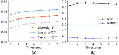
In dynamic graph learning with hyperbolic geometry, we can assume that the graph is gradually scattered to fully leverage the expansive nature of hyperbolic space. This will lead to an increase in the distance dc between any two nodes yt and zt. Hence, the lower bounds of two errors will also rise over time. To clarify our assumption, we conduct an experimental investigation of the HTGN on the Disease dataset [Bjørnstad et al., 2002].
The Fig. 1a plots the ϵlog t and ϵexp t , which are computed as averaging the errors in Eq. (8) and Eq. (9) for each snapshot Gt. The distortion error ϵt is denoted as the average of ϵlog t and ϵexp t . As the errors depend on the mean pairwise distance (MPD) among nodes in the hyperbolic space and the mean maximum distance to the origin point of the manifold (MMDO), we also give their plots in Fig. 1b. Because HTGN uses a fixed reference point, the term (1-c∥xt∥) is constant. The MPD, correlating with the pairwise distance dc in the error bound, slightly increases over time. Meanwhile, the MMDO, correlating with the term α in the error bound, gradually decreases. When the graph grows over time, the three error terms ϵt, ϵlog t and ϵexp t grow linearly, which reduces the learning capability of HTGN in general.
4 Method
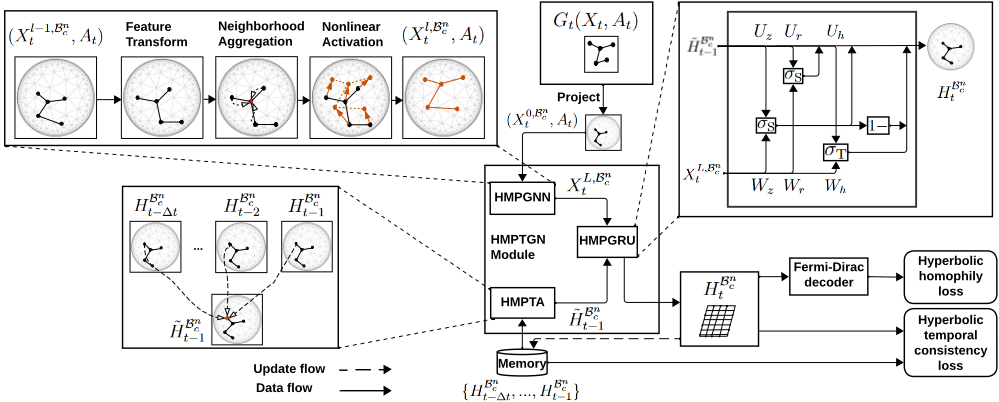
To avoid the distortion caused by tangent space, we propose the Hyperbolic Manifold-Preserving Temporal Graph Network (HMPTGN) that fully operates on the hyperbolic manifold. As illustrated in Fig. 2, our HMPTGN comprises three components: (i) HMPGNN - a graph neural network to capture spatial relationships within the hyperbolic space; (ii) HMPTA - a temporal attention mechanism to generate an informative historical state; (iii) HMPGRU - a recurrent unit to compute the output from the spatio-temporal features. Based on the graph recurrent framework [Yang et al., 2021], each module is designed to learn relevant information to model the evolution of dynamic graphs. Moreover, by utilizing the Mobius addition, the Klein model, and the Poincar´e linear transformation, the manifold-preserving property can be guaranteed in each of the three modules in HMPTGN.
4.1 Hyperbolic Manifold-Preserving Graph Neural Network
The HMPGNN module extends the standard messagepassing framework from the Euclidian space to the hyperbolic manifold. As input graph snapshot Gt(Xt, At) is represented in the Euclidean space, it is firstly needed to project to the hyperbolic space via Eq. (7). The resulting hyperbolic representation Gt(XBn c t ,At) is then passed through L layers of the HMPGNN module. The lth layer in HMPGNN receives the output Xl-1,Bn c t from the previous layer to produce the new node features Xl,Bn c t . The initial hyperbolic representation of Gt is denoted as X0,Bn c t . As shown in Fig. 2, each lth layer includes a feature transformation, a neighborhood aggregation, and a nonlinear activation.
Hyperbolic feature transformation. The feature transformation in Euclidean GCNs is a linear transformation based on normal matrix-vector multiplication. However, applying normal matrix-vector multiplication in hyperbolic space does not ensure that the transformed nodes reside on the manifold. To address this, we develop a Poincar´e linear transformation, denoted by ⊗c as follows:
where x is a node embedded on the Poincar´e ball Bn c , W is an orthogonal matrix, and I is an identity matrix. The manifoldpreserving property of the Poincar´e linear transformation is proved in Proposition 1.
Proposition 1. The Poincar´e linear transformation ensures that the output node y lies on the Poincar´e ball.
Now, we can apply the Poincar´e linear transformation to the node feature in hyperbolic space directly:
where W l , bl are trainable parameters and xl,Bn c t,i is the representation of node i at layer l on the manifold Bn c , i.e. Xl,Bn c t = {xl,Bn c t,i }i=|Vt| i=1 . For the bias addition ⊕c with parameter bl , the M¨obius addition in Eq. (3) is employed. To learn the constrained parameter W l effectively, we follow the work of [Lezcano-Casado, 2019].
Hyperbolic neighborhood aggregation. We utilize the Einstein midpoint [Ungar, 2005] in the Klein model as our aggregate function. Firstly, we map each node representation zl,Bn c t,i obtained by the hyperbolic feature transformation in Eq. (11) to the Klein model via operation pBn c →Kn c in Eq. (5). Then we compute the aggregated representation of each node i as the weighted Einstein midpoint:
where γj = (1 - c∥zl,Kn c t,j ∥2 )-1/2 is the Lorentz factor, wij = ((deg(j) + 1)(deg(i) + 1))-1/2 is the normalized weight from GCN [Kipf and Welling, 2016a], deg(i) is the degree of node i, N(i) is the neighborhood of node i, zl,Kn c t,j is the representation of node j in the Klein model. Finally, for each node i, the output ˜ zl,Kn c t,i is projected back to the Poincar´e ball by the reverse mapping pKn c →Bn c in Eq. (5). In comparison to H2H-GCN [Dai et al., 2021], our version includes an addition weight normalization trick to avoid exploding and vanishing gradient issues.
Hyperbolic nonlinear activation. The hyperbolic activation is given by:
The possible choices of σ include ReLU, Sigmoid, Tanh denoted as σR, σS, σT respectively. If we assume the input and output of the activation function are bounded, the following proposition guarantees that our HMPGNN is manifoldpreserving on the Poincar´e ball Bn c .
Proposition 2. Given z such that ∥z∥2 < α and a nonlinear activation σ, such that ∥σ(z)∥2 < β , for known constants α , β > 0. There exists a Poincar´e ball Bn c that z ∈ Bn c and σ(z) ∈ Bn c .
Given the input and output of Eq. (13), it can be shown that all of the σR, σS, σT satisfy the manifold-preserving property. In practice, for training stability, one can increase the radius value of the Poincar´e ball Bn c to ensure the manifoldpreserving property of σ.
By combining the feature transformation, neighborhood aggregation, and nonlinear activation, each layer of the HMPGNN module ensures that the output embedding stays on the Poincar´e ball. After going through L layers of HMPGNN, we get the final node representation XL,Bn c t = {xL,Bn c t,i }i=|Vt| i=1 that contains the intact spatial structure information of the snapshot Gt in hyperbolic space.
4.2 Hyperbolic Manifold-Preserving Temporal Attention
To model the historical evolutionary information, we employ HMPTA, a temporal attention layer over a time window with fixed-length ∆t. This approach is well-known for learning in dynamic graphs such as HGWaveNet [Bai et al., 2023]. However, our proposed attention architecture is designed to work directly on the hyperbolic manifold instead of the tangent space, by using the Einstein midpoint.
Given a set of historical states of ith node {hBn c τ,i }τ=t-1 τ=t-∆t as the input, the temporary historical state ˜hBn c t-1,i is computed as follows. Firstly, we compute the attention coefficient µi across different historical states:
where the weight matrix Q and vector r are trainable, and ∥ is the concatenate operation. Then we apply the Einstein midpoint to achieve the final hidden state:
where γτ = (1-c∥hKn c t-τ,i ∥2 )-1/2 is the Lorentz factor, hKn c t-τ,i is the corresponding embedding of the historical state hBn c t-τ,i after projecting to the Klein model via pBn c →Kn c in Eq. (5). Lastly, we project the output ˜hKn c t-1,i to the Poincar´e ball via pKn c →Bn c in Eq. (5), to achieve the historical state ˜hBn c t-1,i .
The work of DHGAT [Li et al., 2023] also utilizes the Einstein midpoint for temporal attention. However, DHGAT computes weights using hyperbolic distances between each pair of snapshots, resulting in a memory complexity of O(|Vt|∆t2d), where d is representation dimension. In contrast, our HMPTA with the attention weights in (15) are computed on the linear memory Mi and has a memory complexity of O(|Vt|∆td).
4.3 Hyperbolic Manifold-Preserving Gated Recurrent Unit
By leveraging the Poincar´e linear transformation in Eq. (13), we propose HMPGRU, a recurrent unit that works without tangent space, which is illustrated in Fig. 2. More formally, the HMPGRU module outputs the hidden representation HBn c t of the snapshot Gt using input pair (XL,Bn c t , ˜HBn c t-1 ), where XL,Bn c t represents the node features achieved from the
Algorithm 1 HMPTGN learning process
Input: List of snapshots {Gt(Xt,At)}t=T t=1
Output: List of hidden representations {HBn c t }t=T t=1
- 1: Initialize memory ∆t ×{HBn c 0 } and curvature c
- 2: for t = 1 to T do
- 3: X0,Bn c t = expc0 (Xt)
- 4: XL,Bn c t = HMPGNN(X0,Bn c t , At)
- 5: ˜HBn c t-1 = HMPTA(HBn c t-1 ; ...; HBn c t-∆t )
- 6: HBn c t = HMPGRU(XL,Bn c t ; ˜HBn c t-1 )
- 7: Lt = Lt,c +λLt,r
- 8: Minimize Lt
- 9: Update memory
- 10: end for
- 11: return {HBn c t }t=T t=1
HMPGNN module and ˜HBn c t-1 represents the temporary synthetic historical state from HMPTA module.
The update gate P Bn c t and the reset gate RBn c t at timestamp t of HMPGRU, which balance the input and the memory, are computed as:
The current memory state ˜HBn c t using the reset gate to store the relevant information from the past, is calculated as:
The output latent representation HBn c t is then combined from the synthetic memory state and the current memory state:
where Wz, Wr, Wh, Uz, Ur, Uh are the weight parameters, and ⊙ is the Hadamard product. Following the properties of the Sigmoid σS and Tanh σT functions in Proposition 2, all hidden representations P Bn c t , RBn c t reside on the Poincar´e ball. Moreover, the manifold-preserving property of the Hadamard product is given by the following proposition:
Proposition 3. Given x, p ∈ Bn c such that 0 ≤ pi ≤ 1 ∀i = 1, .., n. Then we have x ⊙ p ∈ Bn c .
Using this property of Hadamard product, it is straightforward to show that the output HBn c t in (16) stays on the Poincar´e ball.
4.4 Overall Framework of HMPTGN
We summarize the HMPTGN learning process in Algorithm 1. Given a collection of snapshots {Gt(Xt,At)}t=T t=1 as the input, we want to extract contextual representations {HBn c t }t=T t=1 which can be used to learn downstream tasks such as link prediction and new link prediction. Firstly, the memory states and the curvature of the Poincar´e ball are initialized. The memory stores hidden representations of ∆t snapshots before Gt. Let 0 be the origin point of the Poincar´e ball Bn c . For each snapshot Gt, the Euclidean node features Xt, which is assumed to be in T0Bn c , is mapped to the Poincar´e ball Bn c via Eq. (7). Then the acquired node representation X0,Bn c t is sent to an L-layer HMPGNN unit. At the same time, multiple historical states from the memory {HBn c τ }τ=t-1 τ=t-∆t are aggregated in HMPTA to achieve the temporary historical state ˜HBn c t-1 . Finally, the outputs XL,Bn c t and ˜HBn c t-1 are given to HMPGRU to produce the hidden representation HBn c t .
We employ the objective function Lt in [Yang et al., 2021] for training HMPTGN. The proposed Lt is a weighted combination of the two losses: Hyperbolic temporal consistency Lt,c to ensure the temporal smoothness and long-term prediction ability; and Hyperbolic homophily loss Lt,r to maximize the probability of linked nodes through the hyperbolic features and minimize the probability of no interconnected nodes.
5 Experiments
5.1 Experiment Setup
Datasets. We evaluate our model and other baselines on 6 datasets: email communication networks Enron [Klimt and Yang, 2004]; academic co-author networks (COLAB) [Yang and Leskovec, 2012]; private messaging network system among students (UCI) [Panzarasa et al., 2009]; synthetic dataset based on the SIR disease spreading model (Disease) [Bjørnstad et al., 2002]; interactions network on the Math Overflow website (MO) [Paranjape et al., 2016]; social network graph of FacebookWall posts (FB) [Yang et al., 2021].
Baselines. We compare the performance of HMPTGN with recent dynamic graph embedding methods in both Euclidean and hyperbolic space. Euclidean approaches include DySAT [Sankar et al., 2018], EvolveGCN [Pareja et al., 2019] VGRNN [Hajiramezanali et al., 2020], and GRUGCN proposed in [Yang et al., 2021], while hyperbolic approaches consist of HTGN [Yang et al., 2021], HGWaveNet [Bai et al., 2023] and DHGAT [Li et al., 2023]. We also implement the HGRUHGCN model as a lightweight extension of GRUGCN by replacing GRU and GCN with Hyperbolic GRU and Hyperbolic GCN. Our implementation is available at the github repository https://github.com/quanlv9211/HMPTGN.
Evaluation Tasks and Metrics. Following HTGN [Yang et al., 2021], we evaluate our HMPTGN on two downstream tasks: temporal link prediction and temporal new link prediction. In temporal link prediction, the model has to predict the edges that appear in {Gt+1,Gt+2, ...} after being trained on {G1,G2, ...,Gt}. Meanwhile, temporal new link prediction aims to predict edges in Gτ but not in Gτ-1 for any snapshot index τ > t. The reported metrics care about average precision (AP) and area under the ROC curve (AUC). We choose the last k snapshots as the test set and the rest as the training set. To ensure a balanced measurement, we consider all edges within the test set as true and randomly sample an equivalent number of unconnected edges as false.
5.2 Experimental Results
We run the experiments with three different seeds and report the average value with standard deviation on the test sets in Table 1 and 2. The best results are in bold and the second-best results are in underline for each dataset.
Temporal link prediction. It can be clearly seen that our proposed model outperforms the competing methods on most datasets on both learning tasks, including non-hyperbolic and hyperbolic approaches. Only the recent HGWaveNet has slightly better results than the HMPTGN in the UCI dataset, while the former achieves lower performances on the remaining datasets. On very large graphs (e.g. MO, FB), DHGAT suffers from the out-of-memory (OOM) problem because of the memory complexity in its temporal attention function. Meanwhile, our HMPTGN achieves average gains of 1.92% in AUC and 1.93% in AP compared to the best baseline.
Temporal new link prediction The results on temporal new link prediction are shown in Table 2. Note that the new link prediction task is more challenging since it requires the model to classify a link that only appears in future snapshots. Our model consistently outperforms the other baselines on most datasets. Moreover, in the Disease benchmark, our model has a significant improvement, gaining 10.32% in AUC and 13.48% in AP compared to the second-best baseline. One of the main reasons is the Disease dataset has a well-defined hierarchical structure. Besides, it has many unseen nodes and edges in the test set, which makes the distortion error more critical to the hyperbolic-based representation.
5.3 Ablation Study
We additionally perform an ablation study to highlight the superiority of the manifold-preserving property in the main components of HMPTGN. Firstly, we create three variants of HMPTGN, which are w/o HMPGNN, w/o HMPTA, and w/o HMPGRU. The three variants are created by removing the manifold-preserving property in that specific component and relying on tangent space to learn the embedding. Then, we evaluate these variants on the Disease dataset with three different seeds. The results are reported in Table 3. In general, removing manifold-preserving property in any component would lower the model's performance. w/o HMPGNN leads to a decline in the model's performance by 2% in average. This is because tangent space has distorted the spatial structure of the graph. Meanwhile, changing to w/o HMPTA leads to a significant decrease in the link prediction task. This suggests that the temporal information carried in the previous snapshots is more accurately obtained on the original manifold compared to the tangent space. Similarly, in the case of w/o HMPGRU, the model's performance also drops dramatically in both tasks. The results affirm the superiority of our hyperbolic preserving modules in comparison to their tangent-based counterparts.
6 RelatedWorks
Dynamic Graph Embedding. There exist diverse techniques for embedding dynamic graphs such as matrix factorizationmethods [Rossi et al., 2013] or randomwalkmethods
| Datasets | Disease | Enron | COLAB | UCI | MO | FB | ||||||
|---|---|---|---|---|---|---|---|---|---|---|---|---|
| Metric | AUC↑ | AP↑ | AUC↑ | AP↑ | AUC↑ | AP↑ | AUC↑ | AP↑ | AUC↑ | AP↑ | AUC↑ | AP↑ |
| DySAT | 78.46 ± 3.21 | 72.58 ± 1.68 | 89.28 ± 0.76 | 88.62 ± 1.19 | 79.83 ± 0.80 | 79.08 ± 2.00 | 75.74 ± 5.35 | 82.63 ± 2.75 | 83.23 ± 2.17 | 84.31 ± 1.90 | 67.49 ± 0.21 | 71.02 ± 0.05 |
| EvolveGCN | 69.25 ± 1.43 | 67.59 ± 1.20 | 90.43 ± 0.45 | 92.85 ± 0.22 | 83.16 ± 0.34 | 87.42 ± 0.35 | 85.10 ± 2.40 | 88.08 ± 1.07 | 69.60 ± 2.47 | 75.19 ± 0.06 | 75.59 ± 0.13 | 79.97 ± 0.16 |
| VGRNN | 83.69 ± 0.78 | 79.58 ± 1.76 | 87.89 ± 0.29 | 86.95 ± 0.17 | 77.45 ± 0.52 | 79.11 ± 0.48 | 79.76 ± 0.92 | 82.68 ± 0.73 | OOM | OOM | ||
| GRUGCN | 87.43 ± 1.71 | 86.51 ± 1.70 | 92.16 ± 0.21 | 92.82 ± 0.23 | 83.66 ± 0.19 | 86.27 ± 0.35 | 73.86 ± 1.01 | 81.37 ± 0.45 | 67.70 ± 3.24 | 77.56 ± 2.13 | 78.25 ± 0.56 | 81.36 ± 0.38 |
| HGRUHGCN | 80.56 ± 0.38 | 78.89 ± 0.62 | 91.55 ± 1.42 | 92.14 ± 1.26 | 83.10 ± 0.73 | 87.03 ± 0.37 | 80.97 ± 0.83 | 83.19 ± 1.19 | 59.06 ± 0.32 | 71.26 ± 0.47 | 75.72 ± 0.25 | 76.95 ± 0.39 |
| HTGN | 82.66 ± 1.04 | 75.45 ± 1.94 | 93.38 ± 0.26 | 93.73 ± 0.23 | 87.78 ± 0.52 | 90.17 ± 0.31 | 90.55 ± 0.11 | 90.02 ± 0.34 | 86.08 ± 0.05 | 85.30 ± 0.16 | 82.29 ± 0.09 | 78.38 ± 0.79 |
| HGWaveNet | 83.80 ± 0.43 | 73.59 ± 2.46 | 94.33 ± 0.17 | 94.39 ± 0.14 | 88.23 ± 0.19 | 90.52 ± 0.22 | 91.86 ± 0.16 | 91.92 ± 0.15 | 85.70 ± 0.46 | 85.15 ± 0.55 | 82.12 ± 0.82 | 78.06 ± 1.60 |
| DHGAT | 91.23 ± 0.22 | 89.44 ± 0.40 | 94.27 ± 0.24 | 93.82 ± 0.40 | 89.13 ± 0.80 | 90.98 ± 0.47 | 79.14 ± 0.35 | 81.92 ± 0.30 | OOM | OOM | ||
| HMPTGN(ours) | 91.45 ± 0.42 | 88.23 ± 0.79 | 95.09 ± 0.27 | 95.17 ± 0.21 | 89.51 ± 0.11 | 91.54 ± 0.04 | 91.52 ± 0.48 | 91.89 ± 0.51 | 86.53 ± 0.46 | 86.34 ± 0.29 | 85.02 ± 0.27 | 83.50 ± 0.14 |
| Gain(%) | + 0.24 | - 1.37 | + 0.81 | + 0.83 | + 0.43 | + 0.62 | - 0.37 | - 0.03 | + 0.52 | + 1.22 | + 3.32 | + 2.63 |
| Datasets | Disease | Enron | COLAB | UCI | MO | FB | ||||||
|---|---|---|---|---|---|---|---|---|---|---|---|---|
| Metric | AUC↑ | AP↑ | AUC↑ | AP↑ | AUC↑ | AP↑ | AUC↑ | AP↑ | AUC↑ | AP↑ | AUC↑ | AP↑ |
| DySAT | 75.67 ± 1.78 | 64.49 ± 0.53 | 83.19 ± 0.22 | 82.16 ± 0.65 | 71.27 ± 0.54 | 70.23 ± 1.69 | 71.50 ± 5.18 | 78.68 ± 3.09 | 82.98 ± 2.23 | 84.74 ± 1.93 | 65.89 ± 0.10 | 69.34 ± 0.27 |
| EvolveGCN | 59.05 ± 0.73 | 53.62 ± 0.91 | 83.92 ± 0.21 | 86.11 ± 0.08 | 72.09 ± 0.64 | 76.87 ± 0.65 | 81.91 ± 2.42 | 85.18 ± 0.87 | 71.58 ± 2.38 | 77.01 ± 0.17 | 73.14 ± 0.15 | 77.33 ± 0.18 |
| VGRNN | 82.11 ± 7.34 | 73.75 ± 9.29 | 80.99 ± 1.03 | 78.53 ± 0.33 | 67.85 ± 0.78 | 69.78 ± 0.42 | 75.61 ± 1.74 | 78.72 ± 1.32 | OOM | OOM | ||
| GRUGCN | 61.80 ± 4.22 | 52.15 ± 2.60 | 85.80 ± 0.23 | 86.31 ± 0.33 | 75.43 ± 0.88 | 77.74 ± 1.06 | 70.00 ± 1.04 | 78.48 ± 0.57 | 69.97 ± 2.76 | 79.31 ± 1.83 | 76.69 ± 0.58 | 79.79 ± 0.39 |
| HGRUHGCN | 76.51 ± 6.31 | 64.48 ± 5.59 | 85.53 ± 2.03 | 85.67 ± 1.45 | 74.41 ± 1.39 | 78.32 ± 0.80 | 77.91 ± 0.31 | 80.04 ± 0.29 | 63.29 ± 0.24 | 74.21 ± 0.34 | 74.23 ± 0.37 | 75.27 ± 0.31 |
| HTGN | 77.54 ± 0.86 | 69.50 ± 5.04 | 88.51 ± 0.47 | 87.62 ± 0.50 | 79.98 ± 0.99 | 81.89 ± 0.56 | 88.98 ± 0.34 | 88.24 ± 0.45 | 85.78 ± 0.07 | 85.56 ± 0.10 | 81.03 ± 0.02 | 77.08 ± 0.70 |
| HGWaveNet | 76.34 ± 4.21 | 62.99 ± 4.01 | 89.69 ± 0.15 | 88.60 ± 0.36 | 80.52 ± 0.38 | 82.19 ± 0.55 | 90.06 ± 0.54 | 89.96 ± 0.40 | 85.53 ± 0.40 | 85.45 ± 0.60 | 80.82 ± 0.84 | 76.68 ± 1.54 |
| DHGAT | 79.65 ± 0.63 | 68.46 ± 0.84 | 90.01 ± 0.21 | 87.01 ± 0.58 | 81.52 ± 1.06 | 82.01 ± 0.54 | 76.60 ± 0.31 | 78.85 ± 0.48 | OOM | OOM | ||
| HMPTGN(ours) | 90.58 ± 0.79 | 83.69 ± 0.72 | 90.72 ± 0.50 | 89.23 ± 0.05 | 82.29 ± 0.40 | 84.06 ± 0.21 | 89.23 ± 0.18 | 89.36 ± 0.19 | 86.04 ± 0.40 | 86.39 ± 0.20 | 83.74 ± 0.39 | 81.75 ± 0.19 |
| Gain(%) | + 10.32 | + 13.48 | + 0.56 | + 0.71 | + 0.94 | + 2.76 | - 0.93 | - 0.67 | + 0.30 | + 0.97 | + 3.34 | + 2.46 |
| Task | Link prediction | New link prediction | ||
|---|---|---|---|---|
| Metric | AUC↑ | AP↑ | AUC↑ | AP↑ |
| HMPTGN | 91.45 ± 0.42 | 88.23 ± 0.79 | 90.58 ± 0.79 | 83.69 ± 0.72 |
| w/o HMPGNN | 88.81 ± 0.85 | 85.12 ± 1.20 | 88.54 ± 0.50 | 81.16 ± 0.91 |
| Gain(%) | - 2.89 | - 3.52 | - 2.25 | - 3.02 |
| w/o HMPTA | 83.78 ± 1.08 | 77.57 ± 1.74 | 86.21 ± 0.94 | 81.45 ± 0.70 |
| Gain(%) | - 8.39 | - 12.08 | - 4.82 | - 2.68 |
| w/o HMPGRU | 84.48 ± 1.58 | 80.53 ± 1.82 | 76.00 ± 1.76 | 71.15 ± 1.80 |
| Gain(%) | - 7.62 | - 8.73 | - 16.10 | - 14.98 |
[Nguyen et al., 2018]. Recently, deep learning approaches employ neural networks to extract the topological properties and capture temporal dependencies of dynamic graphs, leading to state-of-the-art performances. For instance, DySAT [Sankar et al., 2018] creates node representation through joint self-attention along the spatial and temporal dimensions. VRGNN [Hajiramezanali et al., 2020] enhances the expressive capability by inputting the node embedding generated by VGAE [Kipf and Welling, 2016b] on each snapshot into the hidden state of a graph recurrent network. EvolveGCN [Pareja et al., 2019] incorporates an RNN to update the parameters of the GCNs [Kipf andWelling, 2016a].
Hyperbolic Graph Embedding. Hyperbolic geometry has been utilized in the static graph domain due to its efficiency for modeling data with latent hierarchies [Chen et al., 2021a; Peng et al., 2021; Chen et al., 2021b; Yang et al., 2023]. Recent works [Liu et al., 2019; Chami et al., 2019] extend graph convolution to hyperbolic space by shifting the aggregate operation to the tangent space, enabling the execution of vector operations and leading to the superior performance. However, it is important to note that a tangent space serves as a first-order approximation of the original space and can potentially cause distortion. [Dai et al., 2021] propose H2H-GCN
working directly on the hyperbolic manifold to keep the geometric structure of the graph. In hyperbolic dynamic graph learning, [Yang et al., 2021] propose HTGN, incorporating hyperbolic GNN and hyperbolic GRU to capture spatial and temporal dependencies in dynamic graphs. HGWaveNet [Bai et al., 2023] employs hyperbolic diffusion graph convolution to obtain the structural information of nodes and uses hyperbolic dilated causality convolution to acquire causal relationships between snapshots. DHGAT [Li et al., 2023] employs a hyperbolic self-attention that operates directly on the manifold. However, DHGAT still relies on the tangent space to conduct feature transformation and nonlinear activation.
7 Conclusion
In this paper, we first analyze the drawbacks of tangent space in hyperbolic dynamic graph learning. The tangent space can weaken the learning capabilities of traditional hyperbolic methods. Therefore, we propose HMPTGN, a hyperbolic dynamic graph method that can work directly on the Poincar´e manifold. The HMPTGN consists of three main components to model spatial and temporal relationships in the dynamic graph. Experiment results on real-world datasets demonstrate that our model surpasses the Euclidean-based and other hyperbolic-based methods. Overall, our proposed approach highlights the efficiency of applying hyperbolic space to model the complexity of discrete-time dynamic graphs. The results can also be extended to incorporate different hyperbolic models beyond the Poincar´e ball for modeling the dynamic graph embedding.
Acknowledgments
This material is based upon work supported by the Air Force Office of Scientific Research under award number FA238622-1-4026.
@inproceedings{ijcai2024p484,
  title     = {Toward a Manifold-Preserving Temporal Graph Network in Hyperbolic Space},
  author    = {Le, Viet Quan and Ta, Viet-Cuong},
  booktitle = {Proceedings of the Thirty-Third International Joint Conference on
               Artificial Intelligence, {IJCAI-24}},
  publisher = {International Joint Conferences on Artificial Intelligence Organization},
  editor    = {Kate Larson},
  pages     = {4380--4388},
  year      = {2024},
  month     = {8},
  note      = {Main Track},
  doi       = {10.24963/ijcai.2024/484},
  url       = {https://doi.org/10.24963/ijcai.2024/484},
}
TY - CPAPER TI - Toward a Manifold-Preserving Temporal Graph Network in Hyperbolic Space AU - Le, Viet Quan AU - Ta, Viet-Cuong T2 - Proceedings of the Thirty-Third International Joint Conference on Artificial Intelligence, IJCAI-24 PB - International Joint Conferences on Artificial Intelligence Organization PY - 2024 SP - 4380 EP - 4388 DO - 10.24963/ijcai.2024/484 UR - https://doi.org/10.24963/ijcai.2024/484 ER -Copied
Machine-readable versions of this paper, for tools and AI agents:





