
Updates on the Complexity of SHAP Scores
Proceedings of the Thirty-Third International Joint Conference on Artificial Intelligence. Main Track. Pages 403-412.
https://doi.org/10.24963/ijcai.2024/45
Keywords
- AI Ethics, Trust, Fairness: ETF: Explainability and interpretability
- AI Ethics, Trust, Fairness: ETF: Trustworthy AI
- Knowledge Representation and Reasoning: KRR: Computational complexity of reasoning
- Machine Learning: ML: Explainable/Interpretable machine learning
Abstract
SHAP scores represent one of the most widely used methods of explainability by feature attribution, as illustrated by the explainable AI tool SHAP.
A number of recent works studied the computational complexity of the exact computation of SHAP scores, covering a comprehensive range of families of classifiers.
This paper refines some of the existing complexity claims, including families of classifiers for which the computation of SHAP scores is computationally hard and those for which there exist polynomial-time algorithms.
- [Arenas et al., 2021] Marcelo Arenas, Pablo Barceló, Leopoldo E. Bertossi, and Mikaël Monet. The tractability of shap-score-based explanations for classification over deterministic and decomposable boolean circuits. In AAAI, pages 6670-6678, 2021.
- [Arenas et al., 2023] Marcelo Arenas, Pablo Barceló, Leopoldo E. Bertossi, and Mikaël Monet. On the com- plexity of shap-score-based explanations: Tractability via knowledge compilation and non-approximability results. J. Mach. Learn. Res., 24:63:1-63:58, 2023.
- [Arora and Barak, 2009] Sanjeev Arora and Boaz Barak. Computational Complexity -A Modern Approach. Cam- bridge University Press, 2009.
- [Bauer and Kohavi, 1999] Eric Bauer and Ron Kohavi. An empirical comparison of voting classification algorithms: Bagging, boosting, and variants. Mach. Learn., 36(1- 2):105-139, 1999.
- [Breiman, 1996] Leo Breiman. Bagging predictors. Mach. Learn., 24(2):123-140, 1996.
- [Breiman, 2001] Leo Breiman. Random forests. Mach. Learn., 45(1):5-32, 2001.
- [Campbell et al., 2022] Thomas W Campbell, Heinrich Roder, Robert W Georgantas III, and Joanna Roder. Ex- act shapley values for local and model-true explanations of decision tree ensembles. Machine Learning with Applica- tions, 9:100345, 2022.
- [Chen and Guestrin, 2016] Tianqi Chen and Carlos Guestrin. XGBoost: A scalable tree boosting system. In KDD, pages 785-794, 2016.
- [Darwiche and Marquis, 2002] Adnan Darwiche and Pierre Marquis. A knowledge compilation map. J. Artif. Intell. Res., 17:229-264, 2002.
- [Datta et al., 2016] Anupam Datta, Shayak Sen, and Yair Zick. Algorithmic transparency via quantitative input in- fluence: Theory and experiments with learning systems. In IEEE S&P, pages 598-617, 2016.
- [Delgado et al., 2014] Manuel Fernández Delgado, Eva Cer- nadas, Senén Barro, and Dinani Gomes Amorim. Do we need hundreds of classifiers to solve real world classifica- tion problems? J. Mach. Learn. Res., 15(1):3133-3181, 2014.
- [Freund and Schapire, 1996] Yoav Freund and Robert E. Schapire. Experiments with a new boosting algorithm. In Lorenza Saitta, editor, ICML, pages 148-156, 1996.
- [Freund and Schapire, 1997] Yoav Freund and Robert E. Schapire. A decision-theoretic generalization of on-line learning and an application to boosting. J. Comput. Syst. Sci., 55(1):119-139, 1997.
- [Freund, 1995] Yoav Freund. Boosting a weak learning al- gorithm by majority. Inf. Comput., 121(2):256-285, 1995.
- [Friedman, 2001] Jerome H Friedman. Greedy function ap- proximation: a gradient boosting machine. Annals of statistics, pages 1189-1232, 2001.
- [Lundberg and Lee, 2017a] Scott M. Lundberg and Su-In Lee. Consistent feature attribution for tree ensembles. CoRR, abs/1706.06060, 2017.
- [Lundberg and Lee, 2017b] Scott M. Lundberg and Su-In Lee. A unified approach to interpreting model predictions. In NeurIPS, pages 4765-4774, 2017.
- [Lundberg et al., 2018] Scott M. Lundberg, Gabriel G. Erion, and Su-In Lee. Consistent individualized feature at- tribution for tree ensembles. CoRR, abs/1802.03888, 2018.
- [Lundberg et al., 2020] Scott M Lundberg, Gabriel Erion, Hugh Chen, Alex DeGrave, Jordan M Prutkin, Bala Nair, Ronit Katz, Jonathan Himmelfarb, Nisha Bansal, and Su- In Lee. From local explanations to global understanding with explainable ai for trees. Nature machine intelligence, 2(1):56-67, 2020.
- [Molnar, 2020] Christoph Molnar. Interpretable machine learning. https://christophm.github.io/ interpretable-ml-book/, 2020. Last accessed: 2024- 06-11. Link
- [Muschalik et al., 2024] Maximilian Muschalik, Fabian Fu- magalli, Barbara Hammer, and Eyke Hüllermeier. Beyond TreeSHAP: Efficient computation of any-order Shapley in- teractions for tree ensembles. In Michael J. Wooldridge, Jennifer G. Dy, and Sriraam Natarajan, editors, AAAI, pages 14388-14396, 2024.
- [Opitz and Maclin, 1999] David W. Opitz and Richard Maclin. Popular ensemble methods: An empirical study. J. Artif. Intell. Res., 11:169-198, 1999.
- [Pedregosa et al., 2011] Fabian Pedregosa, Gaël Varoquaux, Alexandre Gramfort, Vincent Michel, Bertrand Thirion, Olivier Grisel, Mathieu Blondel, Peter Prettenhofer, Ron Weiss, Vincent Dubourg, Jake VanderPlas, Alexandre Pas- sos, David Cournapeau, Matthieu Brucher, Matthieu Per- rot, and Edouard Duchesnay. Scikit-learn: Machine learn- ing in python. J. Mach. Learn. Res., 12:2825-2830, 2011.
- [Ribeiro et al., 2016] Marco Túlio Ribeiro, Sameer Singh, and Carlos Guestrin. "why should I trust you?": Explain- ing the predictions of any classifier. In KDD, pages 1135- 1144, 2016.
- [Ribeiro et al., 2018] Marco Túlio Ribeiro, Sameer Singh, and Carlos Guestrin. Anchors: High-precision model- agnostic explanations. In AAAI, pages 1527-1535, 2018.
- [Roth, 1988] Alvin E Roth. The Shapley value: essays in honor of Lloyd S. Shapley. Cambridge University Press, 1988.
- [Rozemberczki et al., 2022] Benedek Rozemberczki, Lau- ren Watson, Péter Bayer, Hao-Tsung Yang, Oliver Kiss, Sebastian Nilsson, and Rik Sarkar. The shapley value in machine learning. In IJCAI, pages 5572-5579, 2022. IJCAI
- [Sagi and Rokach, 2018] Omer Sagi and Lior Rokach. En- semble learning: A survey. WIREs Data Mining Knowl. Discov., 8(4), 2018.
- [Schapire, 1990] Robert E. Schapire. The strength of weak learnability. Mach. Learn., 5:197-227, 1990.
- [Shapley, 1953] Lloyd S. Shapley. A value for n-person games. Contributions to the Theory of Games, 2(28):307- 317, 1953.
- [Strumbelj and Kononenko, 2010] Erik Strumbelj and Igor Kononenko. An efficient explanation of individual classifi- cations using game theory. J. Mach. Learn. Res., 11:1-18, 2010.
- [Strumbelj and Kononenko, 2014] Erik Strumbelj and Igor Kononenko. Explaining prediction models and individual predictions with feature contributions. Knowl. Inf. Syst., 41(3):647-665, 2014.
- [Van den Broeck et al., 2021] Guy Van den Broeck, Anton Lykov, Maximilian Schleich, and Dan Suciu. On the tractability of SHAP explanations. In AAAI, pages 6505- 6513, 2021.
- [Van den Broeck et al., 2022] Guy Van den Broeck, Anton Lykov, Maximilian Schleich, and Dan Suciu. On the tractability of SHAP explanations. J. Artif. Intell. Res., 74:851-886, 2022.
- [Wegener, 2000] Ingo Wegener. Branching programs and bi- nary decision diagrams: theory and applications. SIAM, 2000.
- [Zhou, 2012] Zhi-Hua Zhou. Ensemble methods: founda- tions and algorithms. CRC press, 2012.
References were extracted automatically from the PDF and may contain errors.
Full text extracted automatically from the PDF; figures, tables and equations may differ. The PDF is the version of record.
1 Introduction
Shapley values [Shapley, 1953; Roth, 1988] are widely used as a method for explaining the prediction of machine learning (ML) models by feature attribution [Molnar, 2020], being referred to as SHAP scores [Strumbelj and Kononenko, 2010; Strumbelj and Kononenko, 2014; Datta et al., 2016; Lundberg and Lee, 2017b; Van den Broeck et al., 2021; Arenas et al., 2021; Rozemberczki et al., 2022; Van den Broeck et al., 2022; Arenas et al., 2023].
The computational complexity of computing SHAP scores has been studied in recent years [Van den Broeck et al., 2021; Arenas et al., 2021; Van den Broeck et al., 2022; Arenas et al., 2023], and the existing intractability results justify the use of incomplete methods for approximating the SHAP scores [Lundberg and Lee, 2017b] for most families of classifiers. There are however exceptions, i.e. there exist families of classifiers for which the computation of SHAP scores has been shown or claimed to be tractable. One well-known example are deterministic decomposable negation normal forms (d-DNNFs), 1 for which polynomial-time algorithms have been devised [Arenas et al., 2021]. Subsequent work generalized those algorithms to classifiers with non-binary discrete features [Arenas et al., 2023]. Furthermore, independent work [Van den Broeck et al., 2021; Van den Broeck et al., 2022] claimed a number of additional (and related) tractability results, namely: (i) Linear regression models; (ii)
1 Which include binary decision trees and free binary decision diagrams [Wegener, 2000; Darwiche and Marquis, 2002].
Decision and regression trees; (iii) Random forests or additive tree ensembles; (iv) Factorization machines, regression circuits; (v) Boolean functions in d-DNNF, binary decision diagrams; and (vi) Bounded-treewidth Boolean functions in CNF. Regarding random forests (and tree ensembles), similar claims have been made in a growing number of works by other authors [Lundberg and Lee, 2017a; Lundberg et al., 2018; Lundberg et al., 2020; Campbell et al., 2022; Muschalik et al., 2024].
As this paper demonstrates, claim (iii) does not hold true when random forests (or tree ensembles) are used for classification, and when class selection is implemented by weighted or majority voting, as is the case with most publicly available implementations. Moreover, this paper proves that the computational complexity of SHAP scores is #P-hard for these widely used families of random forest (RF) classifiers. In order to prove this result, this paper proposes rigorous formalizations of different types of random forests and tree ensembles. More importantly, proposed implementations [Lundberg and Lee, 2017a; Lundberg et al., 2018; Lundberg et al., 2020] are necessarily problematic in the case of RFs/TEs used in practice; otherwise, it would be the case that #P = FP 2 and therefore P = NP [Arora and Barak, 2009].
Furthermore, the paper proposes a generalization of the polynomial-time algorithms for computing SHAP scores proposed in earlier work [Arenas et al., 2021; Arenas et al., 2023], for boolean classifiers defined on binary and nonbinary discrete features, and represented with (non-binary) d-DNNFs. Concretely, the paper extends these algorithms for computing SHAP scores to the case of non-boolean classes, i.e., discrete classifiers, provided the classifiers are represented as generalized d-DNNFs. An immediate consequence of this result is that SHAP scores can also be computed for discrete classifiers represented as read-once decision trees.
The paper is organized as follows. Section 2 introduces the definitions and notation used throughout the paper, including the computation of SHAP scores. Section 3 briefly overviews existing complexity results regarding the computation of SHAP scores. Section 4 formally defines random forests and tree ensembles, and proves basic relationships between different families of tree ensembles. Section 5 proves that computing SHAP scores for the simplest model of random forest is #P-hard. Section 6 shows how to generalize existing polynomial-time algorithms for (binary) d-DNNFs defined on non-binary features [Arenas et al., 2023] to the case of non-boolean classifiers. Section 7 summarizes the paper's contributions.
2 The paper assumes basic knowledge of computational complexity. The complexity classes mentioned in the paper are standard in reference texts [Arora and Barak, 2009].
2 Preliminaries
Classification problems. Let F = {1, . . . ,m} represent a set of features and K = {c1, . . . , cK} represent a set of classes. Each feature i takes values from a domain Di. If feature i is binary, then Di = B = {0, 1}. Similarly, if the classification problem is boolean, then K = B. Both the features' domains and the classes are assumed to be numeric. Given the features' domains, feature space F is defined by F = D1 × D2 × · · · × Dm. A classification function κ maps each point in feature space F to a class in K. One often assumes that κ is non-constant, but this will not be imposed in this paper. A classifier is a tuppleM= (F, F,K, κ). An instance is a tuple (v, c), with v ∈ F representing the input, and c ∈ K, representing the computed output, c = κ(v). Most of the results in Sections 3 and 5 consider binary features and a boolean classification problem. The other sections consider the more general setting where features and classes are nonbinary but discrete.
Finally, the goal of explainability is to find explanations given some instance (v, c). An explanation problem is a tuple E = (M, (v, c)). The paper considers explanations by feature attribution [Molnar, 2020], with another alternative being explanations by feature selection [Molnar, 2020].
Decision trees & ensembles. A decision tree T is a directed acyclic graph composed of a set V of n nodes N = {1, . . . , n} and a set of n - 1 edges E = {e1, . . . , en-1}, where each ei ∈ N × N. By convention, the root node is assigned node number 1, and has no input edges. All other nodes have exactly one input edge. V is partitioned into a set N of non-terminal nodes and a set T of terminal nodes. Each terminal node has no output edges, whereas non-terminal nodes have 2 or more output edges. Each terminal node is associated with a class c ∈ K. Moreover, each non-terminal node p ∈ N is associated with a feature i ∈ F, such that each of the output edges is ascribed a literal (i.e. xi = vi), and while guaranteeing that the literals of the output edges partition the domain of feature i associated with node p. A decision tree T is read-once if along any path of T a feature is associated with at most one node.
Moreover, tree ensembles (TEs) are aggregations of decision trees, equipped with a mechanism for selecting a class for each assignment to the features and given the individual predictions of the decision trees. One example of a widely used mechanism is majority voting [Breiman, 2001; Zhou, 2012]. TEs are discussed in greater detail in Section 4.
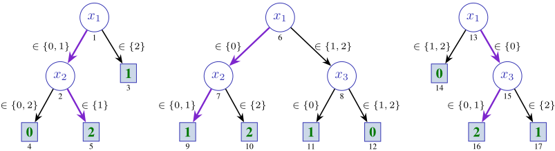
Example 1. Fig. 1 shows the running example of a random forest with majority voting [Breiman, 2001; Zhou, 2012]. For each input, each tree selects the class consistent with the input. The choices of all trees are then combined, and the class selected by most trees is output. The example RF T consists of 3 decision trees T1, T2 and T3, and captures a classification function defined on the F = {1, 2, 3} with Di = {0, 1, 2}, i ∈ {1, 2, 3} and K = {0, 1, 2}. For the input v = (0, 1, 1), tree T1 selects class 2, tree T2 selects class 1, tree T3 selects class 2. Since class 2 is the most selected, then it is the class that is output. The highlighted edges in Fig. 1 indicate the prediction of each tree.
SHAP scores. Methods of eXplainable AI (XAI) can be broadly categorized as those based on feature selection, e.g. Anchors [Ribeiro et al., 2018], and those based on feature attribution, e.g. LIME [Ribeiro et al., 2016] and SHAP [Lundberg and Lee, 2017b]. At present, SHAP and its variants are one of the most widely used explainability approaches.
SHAP is based on the computation of SHAP scores, which represent Shapley values [Shapley, 1953] in the context of explainability [Strumbelj and Kononenko, 2010; Strumbelj and Kononenko, 2014; Lundberg and Lee, 2017b]. We briefly overview the computation of exact SHAP scores, and adopt the formalization of SHAP scores used in recent work [Arenas et al., 2021; Arenas et al., 2023].
Given a point v in feature space F, we define Υ : 2F → 2F as follows,
i.e. for a given set S ⊆ F, and parameterized by the point v in feature space, 3 Υ(S) denotes all the points x = (x1, . . . , xm) ∈ F that have in common with v = (v1, . . . , vm) ∈ F the values of the features specified by S. Using the proposed definition for Υ, we introduce ϕ :
2F → R as follows,
As a result, and given a set S of selected features, ϕ(S) represents the expected value of the classifier over the points of feature space represented by Υ(S). The formulation presented in earlier work [Arenas et al., 2021; Arenas et al., 2023] allows for different input distributions when computing the expected values. For the purposes of this paper, it suffices to consider solely uniform input distributions, and so the dependency on the input distribution is not accounted for.
To simplify the notation, the following definitions are used,
Finally, let Sc : F → R, i.e. the SHAP score for feature i, be defined by,
Given an instance (v, c), the SHAP score assigned to each feature measures the contribution of that feature with respect to the prediction [Strumbelj and Kononenko, 2010].
3 Throughout the paper, all parameterizations are elided for simplicity; these are always clear from the context.
As proved in earlier work [Arenas et al., 2021; Arenas et al., 2023], the definition of SHAP scores (5) can be rewritten as follows:
where, with a slight abuse of notation, we define ς(k) = k!(m-k - 1)!/m!. (6) differs from (5) in that the computation of the SHAP score is organized by different values of k. This modification is instrumental for devising polynomialtime algorithms for computing SHAP scores in the case of d-DNNFs [Arenas et al., 2021; Arenas et al., 2023].
Finally, SHAP Scores denotes the function problem of computing the SHAP scores, given some explanation problem, i.e. a tuple (M, (v, c)), representing a classifier Mand an instance.
3 Complexity of Computing SHAP Scores
Tractable cases. For d-DNNFs, it has been shown that SHAP scores can be computed in polynomial-time for binary classifiers defined on binary features [Arenas et al., 2021]. More recently, this result has been extended to discrete nonbinary features [Arenas et al., 2023]. The downsides of this work are: (i) it applies only to binary classifiers, i.e. classifiers for which the set of classes is {0, 1}; (ii) the circuits are read-once, i.e. in the case of DTs, a feature is tested at most once in each path; and (iii) features are discrete.
Independent work proved that SHAP scores can be computed in polynomial-time for the following families of models [Van den Broeck et al., 2021; Van den Broeck et al., 2022]:
- Linear regression models;
- Decision and regression trees;
- Random forests or additive tree ensembles;
- Factorization machines, regression circuits;
- Boolean functions in d-DNNF, binary decision diagrams; and
- Bounded-treewidth Boolean functions in CNF.
Regarding claim iii. above (which is taken from [Van den Broeck et al., 2021; Van den Broeck et al., 2022]), for random forests and/or additive tree ensembles, the proof of polynomial-time computation of SHAP scores hinges solely on the linearity of expectation [Van den Broeck et al., 2022], and the proof implicitly assumes a regression setting. Unfortunately, and for classification problems, the best-known and most widely used mechanisms for class selection do not respect linearity (see Section 4). 4 Thus, as shown in Section 5, by considering variants of RFs widely used in practice [Breiman, 2001; Pedregosa et al., 2011], the computation of SHAP scores is shown be #P-hard. In turn, this implies that is would be extremely unlikely that the computation of SHAP scores might be polynomial in the case of realistic RFs/TEs classifiers.
Intractable cases. For most families of models it is known that the computation of SHAP scores is intractable, being #Phard [Van den Broeck et al., 2021; Van den Broeck et al., 2022]:
- Logistic regression models;
- Neural networks with sigmoid activation functions;
- Naive Bayes classifiers, logistic circuits; and
- Boolean functions in CNF or DNF.
4 RandomForests &Tree Ensembles
In order to prove complexity results regarding random forests (RF) and tree ensembles (TE) classifiers, we must first define rigorously how these families of classifiers are organized.
Random forests were originally proposed by Breiman [Breiman, 2001], and targeted the selection of a class by selecting the most voted class from a number of decision trees, each of which built by random selecting the features to consider. More recently, random forests implement a more general organization, in which each tree votes not only a class but assigns a weight to its vote. This weighted voting approach is used for example in Scikit-learn [Pedregosa et al., 2011].
In a more general setting, tree ensembles, 5 capture a fairly general mechanism of aggregating weak classifiers (often decision trees) into a single (stronger) classifier. In general, tree ensembles comprise different families of random forests [Breiman, 2001; Pedregosa et al., 2011], boosted trees
4 It should be underlined that both random forests and other tree ensembles are ubiquitous in classification [Breiman, 2001; Zhou, 2012; Delgado et al., 2014; Sagi and Rokach, 2018].
5 Ensembles of classifiers have been studied extensively over the years [Schapire, 1990; Freund, 1995; Breiman, 1996; Freund and Schapire, 1996; Freund and Schapire, 1997; Opitz and Maclin, 1999; Zhou, 2012; Sagi and Rokach, 2018].
(BTs) [Friedman, 2001; Chen and Guestrin, 2016], among many others [Zhou, 2012; Sagi and Rokach, 2018].
This section formalizes TE, BT and different types of RF classifiers. In addition, this section also proves some of their relationships.
General case for TEs. A TE E represents a set of decision trees T(E) = {T1, . . . , Tk}. Each tree Tj consists of a set of paths {P1,j, . . . , Prj,j} such that for each input x ∈ F, exactly one path is consistent with x. Moreover, for each input x ∈ F, each Tj tree outputs a class c(Tj, x) ∈ K and a weight w(Tj , x) ∈ R, to be assigned to the picked class c. By summing up the weights of each class over all trees, the class with the largest sum of weights is the predicted class.
For each class cr ∈ K, its assigned weight is defined as follows:
where ITE denotes the if-then-else operator. Finally, the picked class, given the input x is given by,
Boosted trees [Chen and Guestrin, 2016]. Boosted tree (BTs) are a special case of a TE such that each decision tree Tj is associated with a pre-defined class c(Tj) ∈ K. In addition, for each input x ∈ F, each tree Tj outputs a weight w(Tj, x), to be associated with the class c(Tj). Given the definition of class and weight associated with the tree, it is plain to redefine (7) and (8) in the case of BTs. Furthermore, it is immediate that a BT is a special case of a TE, and so it is the case that,
Proposition 1. Any BT is a TE.
Proof. We reduce a BT to a TE as follows. For any x ∈ F and any Tj ∈ T, set c(Tj, x) = c(Tj). It is then immediate to compute W(cr, x) given (7), and pick the resulting class using (8).
RFs with weighted voting [Pedregosa et al., 2011]. Random forest with weighted voting (RFwv) output a class and an associated weight for each tree. The selected class is the class with the largest sum over all trees. As can be concluded, each RFwv is a TE and vice-versa.
Proposition 2. Any RFwv is a TE (and vice-versa).
RFs with majority voting [Breiman, 2001]. Random forests with majority voting (RFmv) are based on a fairly restricted model, in that for each point x ∈ F, each decision tree Tj chooses a class c(Tj, x) ∈ K, and the picked class is the class chosen by the majority of the decision trees. Thus, we can rewrite (7) as follows:
Moreover, (8) is also used to pick the selected class in the case of RFmv. Despite the relative simplicity, majority voting ranks as one of the most popular voting methods [Zhou, 2012].
Given the above definition of RFmv, we now prove that, Proposition 3. The following holds:
- Any RFmv is a BT;
- Any RFmv is a RFwv; and
- Any RFmv is a TE.
Proof. We analyze each case separately.
- Any RFmv is a BT: Given a RFmv, we replace each tree Tj by |K| copies. For each class cr ∈ K, copy Tj,r outputs weight 1 if the predicted class if cr; otherwise it outputs weight 0.
- Any RFmv is a RFwv: The reduction mimics the one for the general case below.
- Any RFmv is a TE:
From each tree Tj , we construct a modified decision tree as follows. Each leaf in the original DT Tj, with output class cr, will output a pair (cr, 1) in the resulting TE.
Complexity-wise, Proposition 3 can be used to prove hardness results for BTs, RFwvs and TEs, by proving instead hardness results for RFmvs.
Furthermore, it is plain to conclude that this section covers a rather wide range of possible definitions of RFs, and also of their generalizations, i.e. BTs and TEs. It is also plain that the best-known and the most widely used definitions of RFs are covered by the cases studied in this section [Zhou, 2012; Sagi and Rokach, 2018].
Additional variants. Additional mechanisms for creating ensembles include different variants of bagging and boosting [Schapire, 1990; Freund, 1995; Breiman, 1996; Freund and Schapire, 1996; Freund and Schapire, 1997; Bauer and Kohavi, 1999; Friedman, 2001; Zhou, 2012; Sagi and Rokach, 2018]. For classification problems, all such variants must adopt a mechanism to combine results, and select one of the possible classes [Zhou, 2012]. In the case of using decision trees as the basic (weak) classifier, it is plain that any of these ensemble variants can be cast as special cases of the general tree ensemble framework detailed above.
5 Updates on Intractable Cases
This section proves that computing SHAP scores for any of the TE classifiers discussed in Section 4 (including RFwvs and RFmvs) is #P-hard. Unless P = #P (a very unlikely result), the results in this section challenge recent claims that computing SHAP scores for RF is in P (see Corollary 4 of [Van den Broeck et al., 2021] or Corollary 5 of [Van den Broeck et al., 2022]). This section only analyzes in detail the hardness of computing SHAP scores for RFmvs. However, due to Propositions 1 to 3, any hardness result for RFmvs is also a hardness result for any of the other cases of TEs studied in Section 4.
The decision problem for RFmvs is NP-complete. We start by showing a tight connection between the CNFSAT problem and the problem of deciding prediction 1 for a boolean classifier represented with a RFmv.
Definition 1. The decision problem for an ML classifier is to decide the existence of a point x in feature space such that a target class is predicted, i.e. given c ∈ K, the goal is to decide whether x ∈ F exists such that κ(x) = c.
When referring to the different types of RFs/TEs, we will qualify the different decision problems, e.g. the RFmv decision problem refers to RFs with majority voting.
Proposition 4. The decision problem for RFmvs is NPcomplete.
Proof. Clearly, the decision problem is in NP, i.e. given some input, we can decide in polynomial-time whether the prediction is the target one.
Next, we reduce the CNFSAT problem to the problem of deciding whether an RFmv predicts a concrete class.
Let φ = ς1 ∧ ς2 ∧ · · · ∧ ςt be a CNF formula. For each clause ςq in φ, create one tree than predicts 1 iff the clause satisfied, i.e. if any of its literals is satisfied, the prediction is 1; otherwise the prediction for the tree is 0. In addition, create t - 1 trees, each with a single terminal node 0.
Clearly, if all of the t clauses are satisfied, then the RF picks 1, since t trees have picked 1, and only t-1 can pick 0. Conversely, if at least one clause is falsified, the RF picks 0, since now at least t trees pick 0, and at most t - 1 trees pick 1.
It is plain that the reduction is polynomial on the number of literals of φ.
The construction used in the above proof is illustrated by the following example.
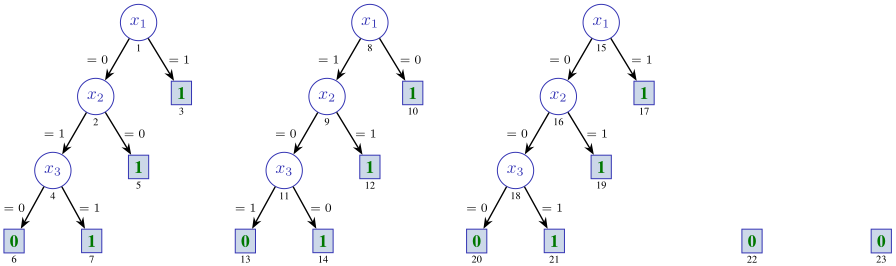
Example 2. Consider the conjunctive normal form (CNF) formula φ = (x1 ∨ ¬x2 ∨ x3) ∧ (¬x1 ∨ x2 ∨ ¬x3) ∧ (x1 ∨ x2 ∨ x3). As illustrated in the proof of Proposition 4, we create one DT for each clause, i.e. three DTs in total. In addition, we create two DTs that just predict 0. As one might antecipate, Fig. 2 represents the reduction of φ to the RF decision problem. Concretely, the formula φ is satisfiable iff there exists a point in feature space for which the prediction is 1.
A possible criticism of the proposed reduction is that the classifier is non-constant iff the formula is satisfiable. (And as noted in Section 2, it is convenient to require the classifier not to be constant.) Nevertheless, one can devise a different reduction, that circumvents this minor issue.
Proposition 5. One can reduce a CNF formula to a nonconstant RFmv classifier such that the predicted class is 1 iff the CNF formula is satisfiable.
Proof. We use classes 0, 1 and 2. Moreover, we add an additional feature xm+1. The semantics becomes as follows:
- If xm+1 = 1, then all DTs are instrumented to output class 2, and so the predicted class is 2. In practice, all the trees above are changed to have a non-terminal root node, that checks the value of xm+1, it picks class 2 if xm+1 = 1, and otherwise, it replicates each of the trees detailed above.
- Clearly, if xm+1 = 0, then the RF behaves as detailed above.
- Moreover, the predicted class is 1 iff φ is satisfiable.
The construction used in the above proof is illustrated by the following example.
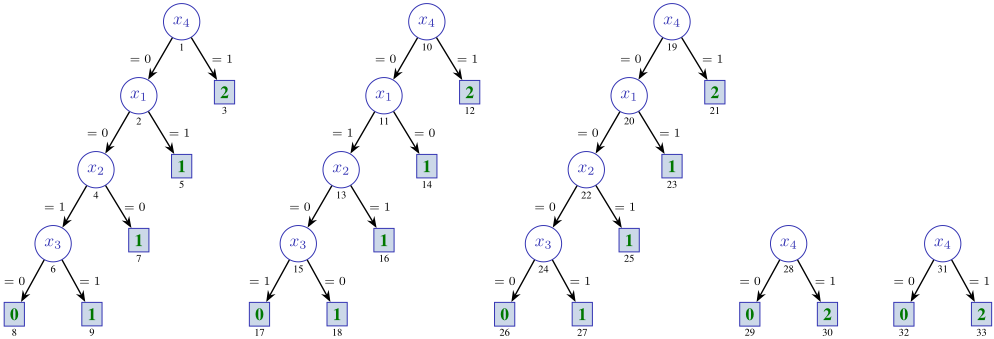
Example 3. We consider again the CNF formula φ from Example 2. Define F = {1, 2, 3, 4} with Di = B, i ∈ {1, 2, 3, 4}, K = {0, 1, 2}. As a result, we construct a random forest with majority voting T = {T1, T2, T3, T4, T5}, as shown in Fig. 3.
SHAP Scores for RFmvs is not in P, unless P = NP. We now exploit well-known properties of SHAP scores, used for example in [Van den Broeck et al., 2022], to disprove a claim also included in [Van den Broeck et al., 2022].
Proposition 6. SHAP Scores for RFmvs is not in P, unless P = NP.
Proof. It is known [Strumbelj andKononenko, 2014; Van den Broeck et al., 2022] that the following holds for SHAP scores:
We show that, if one could compute SHAP scores in polynomial-time for RFmv classifiers, then one could decide SAT in polynomial-time. We proceed as follows:
- Pick any point z in feature space with zm+1 = 0. Then, the predicted class is either 0 or 1. If it is 1, then we are done.
- Otherwise, the prediction is κ(z) = 0, i.e. the predicted class is 0. Let ϕxi (∅), ϕ¬xi (∅) denote, respectively, the average value given the assignments xi = 1, xi = 0. Hence, for any (binary) feature i, it holds that ϕ(∅) = ϕxi (∅)+ϕ¬xi (∅) 2 . Concretely, for i = m + 1, we have ϕxi (∅) = 2, since κ(x) = 2 for any point x with xm+1 = 1. Hence, we get ϕ(∅) = 2 2 + ϕ¬xm+1 2 , and so from (10), we have,
- Clearly, ϕ¬xm+1 = 0 iff the prediction is never 1. Hence, the original formula is satisfiable iff ϕ¬xm+1 ̸= 0, and this we can compute in polynomial-time as long as the SHAP scores can be computed in polynomialtime.
- The previous arguments prove that, if we could compute the SHAP scores of RFs in polynomial-time, then we could decide the satisfiability of a CNF formula in polynomial-time, and so P = NP.
SHAP Scores for RFmvs is #P-hard. As an alternative to the arguments above, we now provide another argument to disprove the claim that SHAP scores for RFmvs is in polynomial-time.
Proposition 7. SHAP Scores is #P-hard.
Proof. From Theorem 3 of [Van den Broeck et al., 2022], it is known that computing the SHAP scores is polynomially equivalent to computing the expected value of a classifier. Furthermore, for a binary classifier, computing the expected value is polynomially equivalent to counting the number of assignments yielding prediction 1.
Now, from the proof of Proposition 4, we observe that for any point x ∈ F, φ(x) = 1 iff κRFmv(x) = 1. Hence, the number of models of φ is the same as the number of points in feature space for which the RF prediction is 1. Thus, if we could count the number of assignments with prediction 1, then we could count the models of a CNF formula, and so SHAP Scores is #P-hard.
SHAP Scores for BTs, RFwvs andTEs are #P-hard. The hardness of computing SHAP scores for BTs, RFwvs and TEs are immediate results given Propositions 1 to 3 and 7.
The corollary of the results in this section is that computing SHAP scores for all of the most widely used TE classifiers (including the simplest type of RF classifiers [Breiman, 2001]) is #P-hard. This means that, for these types of RF and TE classifiers it is extremely unlikely that computing SHAP scores might be in P, as claimed in earlier work, concretely in Corollary 4 of [Van den Broeck et al., 2021] and Corollary 5 of [Van den Broeck et al., 2022]. Similar claims have been made or implied in other works [Lundberg and Lee, 2017a; Lundberg et al., 2018; Lundberg et al., 2020; Campbell et al., 2022; Muschalik et al., 2024], which are also disproved by the results in this section.
6 Update on Tractable Cases
To the best of our knowledge, the only polynomial-time algorithms for computing SHAP scores were proposed for d- DNNFs [Arenas et al., 2021] and later extended to d-DNNFs with non-binary features [Arenas et al., 2023]. 6 In the case of DTs, non-binary d-DNNFs encompass read-once binary decision trees where features can take discrete values. Furthermore, one could conceptually extract an algorithm for a broader range of DTs, by adapting the proof of polynomialtime computation of SHAP scores for decision trees in [Van den Broeck et al., 2021; Van den Broeck et al., 2022]. However, the algorithm extracted from the proof would require solving a system of m equations, which is O(m3 ). In addition, the algorithms proposed in earlier work [Arenas et al., 2021; Arenas et al., 2023] exploit (6) to avoid enumerating all possible sets of fixed features. The purpose of this section is to propose two simple generalizations to the earlier algorithms [Arenas et al., 2021; Arenas et al., 2023], thereby ensuring polynomial-time (and efficient) solutions for computing SHAP scores in the case of d-DNNFs. These generalizations are discussed in the remainder of this section.
6.1 d-DNNF Replication
The first solution consists of analyzing a polynomial number of modified copies of the classifier, each represented by a distinct d-DNNF.
6 As proved elsewhere [Van den Broeck et al., 2021; Van den Broeck et al., 2022], other earlier attempts [Lundberg et al., 2020] resulted in unsound algorithms.
Let γ(x) = ∑l λlκl(x). A well-known result of SHAP scores (e.g. see eq. (4) in [Van den Broeck et al., 2022]) is that,
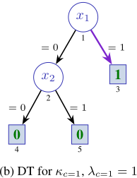
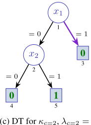
Thus, for a classifier with classes K = {c1, . . . , cK}, we create K copies of the classifier where, for each copy l, the only non-zero prediction is cl, which we set to 1. This becomes function κl and we set λl = cl. Moreover, one then constructs the d-DNNF for the classifier κl, and compute the SHAP scores. Finally, we use (11) to compute the SHAP scores of the original classifier. We refer to this approach as d-DNNF replication.
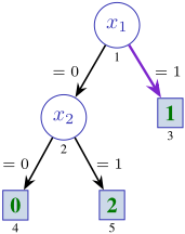
Example 4. For the example DT in Fig. 4a, F = {1, 2, 3}, with Di = B, i = 1, 2, 3 and K = {0, 1, 2}. The target instance is (v, c) = ((1, 1, 1), 1). As noted above, the algorithms proposed in earlier work [Arenas et al., 2021; Arenas et al., 2023] cannot be used for this DT, because K ̸= B. Also, as proposed above, for each cl ∈ K with cl ̸= 1, we create a new d-DNNF representing a classifier for which the only non-zero prediction is for class cl, which we convert to class 1. After computing the SHAP scores, these are multiplied by cl. For the example DT, this is shown in Figs. 4b and 4c. Using Eq. (11), the final computed SHAP scores are obtained by summing over all individual d-DNNFs (DTs in the example), as shown in Fig. 4d.
The discussion above confirms the following result.
Proposition 8. For a classification function γ : F → K that can be expressed as a linear combination of classifiers defined by a linear combination of non-binary but boolean classifiers, each of which represented by a d-DNNF, then the computation of SHAP scores is polynomial-time.
6.2 Non-Binary Non-Boolean d-DNNFs for DTs
The second solution consists of generalizing the non-binary d-DNNFs studied in earlier work [Arenas et al., 2023], to allow for non-binary inputs but also non-boolean classes (NB2) in the concrete case of read-once DTs. The basic algorithm of [Arenas et al., 2023] is included in Appendix A; a few minor changes are clarified below.
We recall that the translation from read-once DTs to dDNNFs is well-known [Arenas et al., 2023]; essentially
| Function | Sc(1) | Sc(2) | λc=cl |
|---|---|---|---|
| κc=1 | 1/2 | 0 | 1 |
| κc=2 | -3/4 | 1/4 | 2 |
| κ | -1/4 | 1/4 |
(d) SHAP scores
Fig. 4: Example of computing SHAP scores for DT, with (v, c) = ((1, 1), 1).
each non-terminal node is replaced by the encoding of an ITE (if-then-else) operator. Concretely, given a node g testing a literal lj, such that the input value is νg,0 when lj is false and νg,1 when lj is true, the output of the node is ITE(lj, νg,1, νg,0), which is encoded in d-DNNFs as OR(AND(lj , νg,1), AND(¬lj , νg,0)).
In contrast to earlier work [Arenas et al., 2021; Arenas et al., 2023], the insight is to allow constant nodes to take any value, subject to constraints on how the d-DNNFs can be organized. In the case of NB2 DTs, ¬-gates are only allowed to have variable nodes as inputs. Moreover, ∧-gates are modified to compute numerical values, given one boolean input and one non-boolean input, i.e. if the boolean input takes value 0, the output is 0, and if the boolean input takes value 1, the output replicates the non-boolean input. Finally, because the d-DNNFs is deterministic, ∨-gates are guaranteed to have at most one input with a non-zero value; this value is replicated to the output. With these restrictions, the algorithms described in earlier work [Arenas et al., 2021; Arenas et al., 2023] can be used without additional changes.
7 Conclusions
This paper revisits recent complexity results regarding the computation of SHAP scores for ML classifiers. The first result proves that an often heralded claim [Lundberg and Lee, 2017a; Lundberg et al., 2018; Lundberg et al., 2020; Van den Broeck et al., 2021; Campbell et al., 2022; Van den Broeck et al., 2022; Muschalik et al., 2024] that SHAP scores for Random Forest (and also Additive Tree Ensemble) classifiers can be computed in polynomial-time does not hold for the most commonly used RF (and TE) classifiers, i.e. those with decision mechanisms based on voting. Concretely, the paper proves that, even for very simple, but realistic, models of RF/TE classifiers, the computation of SHAP scores is #P-hard. A second result refines the class of classifiers for which SHAP scores can be computed in polynomial time. A corollary is that for read-once multi-valued decision trees, the computation of SHAP scores is also polynomial time. A topic of research for decision trees that do not respect the read-once condition is whether SHAP scores can be computed more efficiently than what the proof of membership in P [Van den Broeck et al., 2022] suggests.
Algorithm 1 Computation of SHAP scores for non-boolean DTs
Input: Feature i, Smoothed d-DNNF D with output gout Parameters: Explanation problem E Output: SHAP score Sc(i) 1: function SHAP SCORES(i,D; E) 2: for g ∈ D, by bottom-up induction on D do 3: r ← |var(g) \ {i}| 4: if g is a constant gate with label a then ▷ Constant gate; value of a unrestricted 5: (γ 0 g , δ0 g ) ← (a, a) 6: else if g is a variable gate with var(g) = i then ▷ Variable gate associated with feature i 7: (γ 0 g , δ0 g ) ← (1, 0) 8: else if g is a variable gate with var(g) = j and j ̸= i then ▷ Variable gate not associated with feature i 9: (γ 0 g , δ0 g ) ← (p(j), p(j)) 10: (γ 1 g , δ1 g ) ← (ν(j), ν(j)) 11: else if g is a ¬-gate with input gate g′ then 12: for l ∈ {0, . . . , r} do ▷ Analyze ¬ gate; input gate g′ must be a variable gate 13: q ← (rl ) 14: γ lg ← q - γ lg′ 15: δlg ← q - δlg′ 16: end for 17: else if g is a ∨-gate with input gates g1, g2 then ▷ Analyze ∨ gate, each ∨ gate has a fan-in of exactly 2 18: for l ∈ {0, . . . , r} do 19: γ lg ← γ lg1 + γ lg2 20: δlg ← δlg1 + δlg2 21: end for 22: else if g is a ∧-gate with input gates g1, g2 then ▷ Analyze ∧ gate, each ∧ gate has a fan-in of exactly 2 23: for l ∈ {0, . . . , r} do 24: (r1, r2) ← (|var(g1) \ {i}|, |var(g2) \ {i}|) 25: γ lg ← ∑l1∈{0,...,min(l,r1)},l2∈{0,...,min(l,r2)},l1+l2=l γ l1 g1 · γ l2 g2 26: δlg ← ∑l1∈{0,...,min(l,r1)},l2∈{0,...,min(l,r2)},l1+l2=l δl1 g1 · δl2 g2 27: end for 28: end if 29: end for 30: return ∑m-1 k=0 ς(k) · [(ν(i) -p(i))(γ k gout - δk gout )] ▷ Returned value is the SHAP score Sc(i) for feature i ∈ F 31: end functionA Appendix - SHAP Scores for NB2 DTs
Restriction on d-DNNFs & rationale. We consider dDNNFs obtained from read-once DTs, where features take discrete values, and classes are numerical and discrete, i.e. non-binary features and non-boolean classes (NB2) DTs. The translation from read-once DTs to d-DNNF is wellknown [Arenas et al., 2023]; essentially each non-terminal node is replaced by the encoding of an ITE (if-then-else) operator. Concretely, given a node g testing a literal lj., such that the input value is νg,0 when lj is false and νg,1 when lj is true, the output of the node is ITE(lj, νg,1, νg,0), which is encoded in d-DNNF as OR(AND(lj , νg,1), AND(¬lj , νg,0)).
Building on earlier work [Arenas et al., 2023] we generalize such d-DNNFs to allow for terminal nodes to be assigned arbitrary numerical values. Clearly, the computed value will match the value assigned to the terminal node of the unique path consistent with the input.
Algorithm 1 (see Page 8) summarizes the algorithm for computing SHAP scores for generalized d-DNNFs (e.g. obtained from DTs), which mimics the one proposed in earlier work [Arenas et al., 2023], with minor changes on the requirements on the values of constant nodes. In addition, the algorithm imposes that constant gates must not be the input of ¬-gates. In addition, the value assigned to constant gates is allowed to be arbitrary (see line 4 of Algorithm 1).
Ethical Statement
There are no ethical issues.
Acknowledgments
Part of this work was done while the authors were affiliated respectively with the University of Toulouse and CNRS in France, and it was partially supported by the AI Interdisciplinary Institute ANITI, funded by the French program "Investing for the Future - PIA3" under Grant agreement no. ANR-19-PI3A-0004. X.Huang was also supported in part by the National Research Foundation, Prime Minister's Office, Singapore under its Campus for Research Excellence and Technological Enterprise (CREATE) programme. JMS also acknowledges the extra incentive provided by the ERC in not funding this research.
@inproceedings{ijcai2024p45,
  title     = {Updates on the Complexity of SHAP Scores},
  author    = {Huang, Xuanxiang and Marques-Silva, Joao},
  booktitle = {Proceedings of the Thirty-Third International Joint Conference on
               Artificial Intelligence, {IJCAI-24}},
  publisher = {International Joint Conferences on Artificial Intelligence Organization},
  editor    = {Kate Larson},
  pages     = {403--412},
  year      = {2024},
  month     = {8},
  note      = {Main Track},
  doi       = {10.24963/ijcai.2024/45},
  url       = {https://doi.org/10.24963/ijcai.2024/45},
}
TY - CPAPER TI - Updates on the Complexity of SHAP Scores AU - Huang, Xuanxiang AU - Marques-Silva, Joao T2 - Proceedings of the Thirty-Third International Joint Conference on Artificial Intelligence, IJCAI-24 PB - International Joint Conferences on Artificial Intelligence Organization PY - 2024 SP - 403 EP - 412 DO - 10.24963/ijcai.2024/45 UR - https://doi.org/10.24963/ijcai.2024/45 ER -Copied
Machine-readable versions of this paper, for tools and AI agents:





