AMO-aware Aggregates in Answer Set Programming

1 Introduction

Answer Set Programming (ASP) is a widely adopted formalism for knowledge representation and automated reasoning [Marek and Truszczy´nski, 1999; Niemel¨a, 1999]. In ASP, combinatorial problems are expressed in terms of logic rules comprising several linguistic constructs designed to ease the representation of complex knowledge. Solutions of the represented problem are provided in the form of stable models [Gelfond and Lifschitz, 1990], that is, classical models satisfying an additional stability condition: once the interpretation of the negative literals is fixed according to the model, all the knowledge encoded in the model is required to satisfy the reduced program.

In their simplest form, ASP programs comprise normal rules, each normal rule having a head atom and a body being a conjunction of literals. Intuitively, a head atom is required to be true whenever the associated body is true, so that stable models are classical models of the propositional knowledge base obtained by mapping normal rules to implications (body implies head). The stability condition also enforces other properties of stable models, such as being supported models (every true atom is the head of some rule with true body) [Fages, 1994] and unfounded-free models (the support is acyclic) [Dung, 1992]. All such properties are used to achieve efficient computation by combining a conflict-driven clause learning (CDCL) algorithm [Gebser et al., 2012] with propagators. CDCL is a modern form of non-chronological backtracking based on the pattern choose-propagate-learn

[Marques-Silva et al., 2021]: a branching literal is heuristically chosen and propagated to infer deterministic consequences, where possible, and each inferred literal is associated with a reason being a clause (i.e., a set of literals, one of which is required to be true) among those associated with a propagator. Reasons are used to learn new clauses in case of conflict, so to effectively prune the search space.

Frequently, normal programs are extended by allowing the use of aggregates [Bartholomew et al., 2011; Faber et al., 2011b; Ferraris, 2011; Gelfond and Zhang, 2014; Liu et al., 2010; Simons et al., 2002], in particular SUMs, in rule bodies. In a SUM, Boolean literals are associated with weights, and the sum of the weights of true literals is required to satisfy a given (in)equality. For example, the inequality

(which is satisfied if z = 1 and either x = 1 or y = 1, or x = y = 1 hold) can be enforced by a SUM constraint. There is no general agreement on the stable model semantics of programs extended with arbitrary SUMs [Alviano et al., 2023], but anyhow the results presented in this work apply to the computation of models rather than stable models, and are therefore applicable to any definition of stable model that selects among the classical models of a given program. To simplify the presentation, here we restrict SUMs to be constraints (with nonnegative weights and enforcing the sum of weights to reach a given bound). SUM constraints include at-most-one (AMO) constraints [Surynek, 2020] as special cases, where an AMO essentially inhibits truth of pairs of literals in a given set.

In ASP solvers, SUM (and possibly AMO) constraints are handled by specific propagators [Gebser et al., 2009; Faber et al., 2011a], aiming at delaying the materialization of clauses associated with such constraints. Roughly, the propagator associated with a SUM constraint identifies a literal as necessarily true whenever its weight is required to satisfy the associated inequality. In (1), once z is fixed to 0 (i.e., atom z is assigned false), x = y = 1 is inferred (i.e., atoms x, y are necessarily true). In case of conflict, and only in that case, the clauses {x, z} and {y, z} (i.e., z implies x and y) are possibly materialized if involved in the learning process. A conflict would arise if, for example, x and y are also involved in an AMO constraint, and therefore cannot be both true. In this case, the AMO constraint provides the clause

{x, y}, which is resolved with {y, z} to obtain {x, z} and in turn with {x, z} to obtain the learned clause {z} (i.e., z must be true). It is important to understand that in this example the truth of z is actually logically entailed by the SUM and AMO constraints together (as the learned clause contains z alone). On the other hand, the propagation provided by SUM and AMO independently is insufficient to identify such a deterministic consequence, leading to a more expensive computation to learn such an implicit knowledge in the theory.

This work aims at defining a propagator capable of identifying deterministic consequences of combinations of SUM and AMO constraints. The underlying idea is that literals subject to AMO constraints occurring in a SUM can contribute to the sum of weights up to the largest of their weights rather than the sum of their weights. In the example, x and y can contribute up to 2 (rather than 1 + 2 = 3) to the sum of weights, and therefore truth of z is required to satisfy the inequality. The main research questions addressed by this article are the following:

Q1. What kind of combinations of SUM and AMO constraints are suitable to be jointly processed by a propagator? We identify a promising combination of one SUM constraint and several AMO constraints. Each literal involved in the SUM is also involved in one AMO constraint (possibly being a trivially satisfied singleton), so to reduce the overestimate on the sum of weights and unleash the inference potential of the combined knowledge.

Q2. Is it possible to extend the language with a construct to express such combinations? We provide a new linguistic construct whose syntax extends that of SUM by allowing for specifying a partition of the literals in the SUM, so that each part imposes an AMO constraint.

Q3. How much performance gain can the new propagator provide to an ASP solver? We implemented the proposed propagator and assessed it empirically, reporting performance gain of several orders of magnitude.

2 Preliminaries

This section reports syntax and semantics of normal programs extended with SUM constraints (Section 2.1). Clauses and AMO constraints are given as special cases of SUM (Section 2.2). After that, the stable model search procedure implemented by modern ASP solvers is illustrated with a focus on the concept of propagator (Section 2.3).

2.1 Syntax and Semantics

Let A be a set of atoms. A literal is an atom possibly preceded by the default negation symbol ∼. Given a literal ℓ, ℓ denotes the complement of ℓ, i.e., p = ∼p and ∼p = p for all p ∈ A; for a set L of literals, L is {ℓ | ℓ ∈ L}.

A (normal) rule has the form

where n ≥ 0, p is an atom, and ℓ1, . . . , ℓn are literals. A SUM constraint (or simply constraint) has the form

where n ≥ 0, ℓ1, . . . , ℓn are distinct literals such that ℓi ̸= ℓj (for all 1 ≤ i < j ≤ n), and b,w0, . . . ,wn are nonnegative integers. (We remark here that in ASP-Core-2 standard [Calimeri et al., 2020] the above constraint is written as the headless rule :- #sum{w1, ℓ1 : ℓ1; ...; wn, ℓn : ℓn} < b.) A program is a set of rules and constraints.

Example 1 (Running example). Let Πrun be the following:

Note that there are six atoms (x, y, z, x′ , y′ , z′ ), six rules and two constraints.

We adopt the following notation. Atoms, rules, and constraints occurring in a program Π are respectively denoted as atoms(Π), rules(Π), and constraints(Π). For a rule r of the form (2), H(r) := p (the head atom of r), B(r) := {ℓ1, . . . , ℓn} (the body literals of r), B+(r) := B(r) ∩ A (the atoms occurring in the positive body of r), and B-(r) := B(r) \ A (the atoms occurring in the negative body of r). For a constraint σ of the form (3), let bndσ := b (the bound of σ is b), whσ(ℓi) := wi (the weight of ℓi in σ is wi; for all i ∈ [1..n]), and litsσ := {ℓ1, . . . , ℓn} (the literals occurring in σ are ℓ1, . . . , ℓn). (If σ is clear from the context, it is possibly omitted from the above notation.) Finally, let us define relation ∈ as (wi : ℓi) ∈ σ for i ∈ [1..n], to be read as (wi : ℓi) is an element in (the aggregation set of) σ.

Example 2 (Continuing Example 1). Rule rx is such that H(rx) = x, B+(rx) = ∅ and B-(rx) = {x′ }. Regarding σ2, bndσ2 = 3, wh(y) = 2, y ∈ lits, and (2 : y) ∈ σ2.

An assignment I is a set (or list) of literals such that I ∩ I = ∅; literals in I are true, literals in I are false, and all other literals are undefined. Abusing of notation, let I(ℓ) := 1 if ℓ ∈ I and 0 otherwise (true literals assigned to 1); let I ↑ (ℓ) := 1 if ℓ /∈ I and 0 otherwise (true and undefined literals assigned to 1). Moreover, in the subsequent sections, we will iteratively construct an assignment by using a list and occasionally consider its prefixes (i.e., assignments obtained in previous iterations). I is a (total) interpretation of a program Π if I ∪ I = atoms(Π) ∪ atoms(Π). For total interpretations, relation |= (is model of ) is inductively defined as follows: for a literal ℓ, I |= ℓ if ℓ ∈ I; for a rule r of the form (2), I |= B(r) if I |= ℓ for all ℓ ∈ B(r), and I |= r if I |= H(r) whenever I |= B(r); for a constraint σ of the form (3), I |= σ if ∑ni=1 wi · I(ℓi) ≥ bndσ; for a programΠ, I |= Π if I |= r for all r ∈ rules(Π) and I |= σ for all σ ∈ constraints(Π). The reduct ΠI of a program Π with respect to an interpretation I is {H(r) ← B+(r) | r ∈ rules(Π), I |= r}. (Note that constraints(ΠI ) = ∅.) An interpretation I is a stable model of a program Π if I |= Π and there is no J ⊂ I such that J |= ΠI . Let SM(Π) denote the set of stable models of Π.

Example 3 (Continuing Example 1). We first observe that, in all stable models of Πrun, α′ is true whenever α is false, and vice versa (∀α ∈ {x, y, z}). SM(Πrun) contains {x, y},

{z}, and their supersets (negative literals and prime atoms are omitted for simplicity).

2.2 Clauses and AMO as a Special Cases

Given a set {ℓ1, . . . , ℓn} of n ≥ 0 literals, an at-least-one (ALO) constraint enforces truth of at least one literal in the set. It is also commonly referred to as clause, and can be expressed as the following SUM constraint:

Clause (4) is also written as {ℓ1, . . . , ℓn} (if not ambiguous). Given a set {ℓ1, . . . , ℓn} of n ≥ 1 literals, an AMO constraint inhibits truth of pairs of literals in the set. It can be expressed as the following SUM constraint:

Essentially, it equivalently asks for falsifying all but possibly one literal in the set. In fact, given an interpretation I, I |= (5) if ∑ni=1 I(ℓi) ≥ n - 1, or equivalently ∑ni=1 I(ℓi) ≤ 1. The AMO constraint (5) is compactly written AMO{ℓ1, . . . , ℓn}.

Example 4 (Continuing Example 1). Note that σ1 is the clause {x, y}, or also the AMO constraint AMO{x, y}.

2.3 Stable Model Search and Propagators

Stable model search is implemented in modern ASP solvers using a conflict-driven clause learning (CDCL) algorithm [Gebser et al., 2012]. This algorithm relies on the pattern choose-propagate-learn. In a nutshell, the approach involves incrementally constructing a stable model, starting with an empty list I (representing the empty assignment). During each computational step, a branching literal is heuristically chosen for addition to I. Subsequently, it is propagated to introduce new deterministic consequences to I, where possible. Each deterministic consequence ℓ incorporated into I is associated with a reason being the clause comprising ℓ and the false literals leading to the inclusion of ℓ in I. A conflict arises if the complement of a deterministic consequence is already in I, and its analysis leads to learn new clauses via (backward) resolution starting from the reasons of the conflicting literals. (Recall that resolution combines two clauses {p}∪L and {p}∪L′ to obtain a new clause L∪L′ , where p is an atom, and L, L′ are sets of literals.) During backward resolution, previously added literals are removed from I until the learned clause results in the inclusion of a new deterministic consequence, driving the search into a different branch. This iterative process continues until either I represents a stable model or the empty clause is learned. The latter means that the input program does not admit stable models.

A propagator is a module designed to compute deterministic consequences of a given assignment. The most basic among these modules is unit propagation: a literal ℓ is added to I if there is a clause {ℓ} ∪ L such that L ⊆ I, that is, if ℓ belongs to a clause that can be satisfied only by extending I with ℓ. In this case, reason(ℓ) is defined as {ℓ} ∪ L. Modern ASP solvers enrich the input program with clauses enforcing I to be a model of rules of the form (2) (i.e., {p, ℓ1, . . . , ℓn}), as well as clauses enforcing other required properties of stable models (which are out of the scope of this article).

Example 5. Let Π have, among others, the rules

Hence, a modern ASP solver materializes the clauses

If the current assignment I is the list [w], and z is selected as the branching literal, I is updated to [w, z], and unit propagation infers x, y from the first two clauses, and then y (a conflict) from the third clause. Hence, we have I = [w, z, x, y, y], reason(x) = {x, z}, reason(y) = {y, z}, and reason(y) = {w, x, y}. By resolving reason(y) and reason(y), we obtain {w, x, z}, which still contains more than one atom inferred from the branching point (namely, x and z). By resolving {w, x, z} and reason(x), we obtain {w, z}, which contains only one atom inferred from the branching point (namely, z). CDCL therefore continues with I = [w, z] and reason(z) = {w, z}.

For a SUM constraint σ of the form (3), solvers typically employ a specific aggregate propagator [Gebser et al., 2009; Faber et al., 2011a], which essentially adds to I the literal ℓi (i ∈ [1..n]) if ℓi is required to (possibly) reach the bound b, i.e., if

where J is the first prefix of I meeting the above condition. In this case, reason(ℓi) is {ℓi}∪ (litsσ ∩J), that is, the false literals occurring in σ are enforcing truth of ℓi. In the special case of (5), that is, if σ is AMO{ℓ1, . . . , ℓn}, the literal ℓi (i ∈ [1..n]) is added to I if there is ℓj, with j ̸= i, such that ℓj ∈ I. In this case, reason(ℓi) is {ℓi, ℓj}.

Example 6 (Continuing Example 1). If I is empty, no literal can be inferred from σ1 and σ2. If I is [z], then the application of (6) to the literals of σ2 gives

Hence, x and y are inferred with reason(x) = {x, z} and reason(y) = {y, z}. Note that, once I = [z, x, y], the application of (6) to σ1 gives

Therefore, a conflict is raised, say because y (or similarly x) is added to I with reason(y) = {x, y}.

3 AMOSUMConstraints

In this section, SUM constraints of the form (3) are replaced by the more general AMOSUM constraints (Section 3.1). An AMOSUM constraint combines one SUM constraint with a set of AMO constraints, in a convenient syntax that also results into a more effective propagator (Section 3.2), as formally proved in Section 3.3.

3.1 Syntax and Semantics

An AMOSUM constraint (or simply constraint from this point) σ has the form

where n ≥ 0, ℓ1, . . . , ℓn are distinct literals such that ℓi ̸= ℓj (for all 1 ≤ i < j ≤ n), and b,w0, . . . ,wn, s1, . . . , sn are nonnegative integers. The notation introduced in Section 2.1 is further extended as follows: partsσ := {s1, . . . , sn} (the literals in σ are partitioned into at most n parts s1, . . . , sn), partσ(ℓi) := si (the part of ℓi in σ is si, for all i ∈ [1..n]), and litsσ|s := {ℓ | partσ(ℓ) = s} (the literals in σ belonging to the part s). Moreover, relation ∈ is now defined as (wi : ℓi [si]) ∈ σ for all i ∈ [1..n]. Regarding relation is model of, for σ of the form (7), I |= σ if ∑ni=1 wi · I(ℓi) ≥ bndσ, and ∑ℓ∈litsσ(s) I(ℓ) ≤ 1 for all s ∈ partsσ. Essentially, the definition for (3) is extended by enforcing an AMO constraint on each part of σ.

Example 7 (Continuing Example 1). Πrun is rewritten by replacing σ1 and σ2 with

3.2 Propagation

A constraint σ of the form (7) is associated with three different inference rules. First of all, the AMO inference given by the parts of σ: the literal ℓ is added to I if there is ℓ′ ∈ litsσ|part σ (ℓ) such that ℓ′ ∈ I. In this case, reason(ℓ) is {ℓ, ℓ′ }. The second inference rule is the analogous of the one provided by the aggregate propagator (a literal is inferred true if it is required to reach the bound): the literal ℓ is added to I if J is the first prefix of I such that litsσ|part σ (ℓ) \ J = {ℓ} (ℓ is the last undefined literal in its part), and

where mwhσ(J, s) := max{w · J ↑ (ℓ) | (w : ℓ [s]) ∈ σ} is the maximum weight that part s can contribute to the overall sum. In this case, reason(ℓ) is

where rsnσ(J, ℓ, s) := {ℓ′ } if ℓ′ ∈ litsσ|s ∩ J (i.e., a true literal in the part of ℓ), and {ℓ′ ∈ litsσ|s | whσ(ℓ′ ) > mwhσ(s)} otherwise (i.e., the false literals in the part of ℓ that could had increased the overall sum). The third inference rule has no counterpart in AMO or SUM constraints, and enforces falsity of literals in a part whose weight is guaranteed to be insufficient to reach the bound: the literal ℓ is added to I if J is the first prefix of I such that

In this case, reason(ℓ) is

Example 8 (Continuing Example 7). Already when I is empty, σ3 infers z. In fact, z is the last undefined literal in part 2, and (8) gives

From (9), reason(z) = {z}.

Example 9. Let us consider the following constraint:

If I = [w], the second inference rule associated with σ4 infers z with reason(z) = {z,w}. The same holds if I = [x,w], with the addition of y with reason(y) = {y, x,w}; note that w is included in reason(y) because it could increase the overall sum. On the other hand, if I = [y,w], then x and z are inferred with reason(x) = {x, y,w} and reason(z) = {z,w, y}; note that y is included in reason(z) because it could increase the overall sum (in this specific case y could be ignored, but it is not clear how to efficiently detect such conditions in general). Finally, if I = [x, y,w], then z is inferred with reason(z) = {z,w, x}; in this case, x is included because it enforces a value for part 1 (again, in this specific case it could be ignored).

Example 10. Let us consider the following constraint:

For I = [ ], the third inference rule of σ5 infers x thanks to the application of (10):

In this case, reason(x) = {x}. After that, note that the second inference rule is applicable, and y is inferred with reason(y) = {x, y}.

3.3 Properties

Semantically, it is clear that AMOSUM constraints do not extend the capabilities of the language. In fact, an AMOSUM σ constraint of the form (7) can be expressed in terms of (no more than n + 1) SUM constraints (by design):

On the other hand, it is also true that AMOSUM constraints immediately subsume SUM (and AMO) constraints.

Theorem 1. Every SUM constraint can be expressed by an AMOSUM constraint.

Proof. Let σ be a SUM constraint of the form (3). Construct the following AMOSUM constraint σ′ :

Note that each part s ∈ partsσ′ is a singleton, and therefore trivially satisfies ∑ℓ∈lits σ′ (s) I(ℓ) ≤ 1. Hence, I |= σ if and only if I |= σ′ , for every interpretation I.

The real advantage gained by extending the language with AMOSUM constraints is in the associated inference rules, in particular the second and the third rules (while the first inference rule does not add anything to what can be inferred by AMO constraints). It can be shown that the second inference rule alone is sufficient to capture all deterministic consequences that can be identified by SUM constraints, and actually can result in a larger set of inferred literals.

Theorem 2. Let σ be the AMOSUM constraint of the form (7), σ′ be the SUM constraint of the form (3), and I be an assignment. Let L be the set of literals identified by the second inference rule associated with σ, and L′ be the set of literals inferred by σ′ . Hence, L ⊇ L′ holds, while L′ ⊇ L is not guaranteed.

Proof. Let ℓi be inferred by σ′ (for some i ∈ [1..n]), and let S := partsσ \ {si}. By definition, (6) holds. Hence

and (8) holds as well, proving L ⊇ L′ . A witness of L′ ̸⊇ L is given in Example 8.

Moreover, it is relatively easy to observe that the third inference rule identifies deterministic consequences that are not computed by AMO and SUM constraints. In fact, AMO constraints deal with simple binary inferences, and SUM constraints only infer true literals in their aggregation set (while the third inference rule identifies false literals in the AMOSUM). A witness is given in Example 10.

4 Implementation and Experiments

The propagator outlined in Section 2.2 has been implemented in the ASP solver WASP [Alviano et al., 2015] using its Python interface [Dodaro and Ricca, 2020]. This design choice is motivated by the intuitive interface and its seamless integration into the solver through command line options. In our implementation, AMOSUM constraints are represented by facts, which are interpreted by the Python propagator. Specifically, the representation of an AMOSUM constraint σ of the form (7) is the following:

where group and lb are reserved predicates. Continuing Example 9, σ4 is represented as follows:

Moreover, as WASP already supports efficient propagators for handling AMO constraints, the Python propagator focuses on the other inference rules described in Section 3.2.

The implemented system, referred to as AMOWASP, was assessed empirically against the plain version of WASP [Alviano et al., 2015] v. f3e4c56 and the state-of-the-art system CLINGO v. 5.4.0 [Gebser et al., 2016]. All the tested systems use GRINGO (included in the binary of CLINGO) as grounder. Experiments were executed on an Intel Xeon 2.4 GHz server with 16 GB of memory.

4.1 Benchmarks

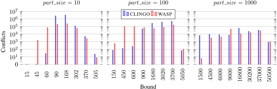
Synthetic Benchmark (SB). Designed to empirically assess the properties outlined in Section 3.3, the first benchmark comprises a program with a rule defining the partition and another one incorporating a SUM aggregate. The partition comprises 10 parts of uniform size part size ∈ {10, 100, 1000}, with the i-th literal of each part having weight i. The bound of the SUM is set to α·C1 (achievable) and C1+α·(C2-C1) (unachievable), where: α ∈ {0.15, 0.45, 0.6, 0.9}; C1 is the sum of the maximumweight in each part, i.e., 10 · part size; C2 is the sumof all weights, i.e., 5·part size ·(part size+1). Hence, the benchmark comprises a total of 24 instances that are trivial for AMOWASP (they are solved without raising any conflict). In contrast, CLINGO and WASP cannot perform the same inferences (see Theorem 2), and we have measured the number of conflicts found by the two systems within the first minute of computation.

GraphColoring (GC). In the Graph Coloring problem, the input consists of a graph and a set of colors, and the objective is to assign a color to each node so that connected nodes do not share the same color. Here, colors are also associated with weights, and the sum of weights is required to reach a certain threshold value. Instances are generated from those employed in the ASP competition [Calimeri et al., 2016], with the colors red, green, blue, yellow, and cyan associated with the weights 2, 4, 8, 16, and 64 to, respectively. For each instance of n nodes, the threshold is set to α · 64 · n, where α ∈ {0.15, 0.45, 0.75}. Time and memory were limited to 20 minutes and 15 GB, respectively.

Knapsack (K). A set of item types is provided, each with an associated weight and value. Additionally, a knapsack capacity and a threshold are given. The objective is to determine whether it is possible to select a specific number of items from each type in such a way that the total weight remains within the knapsack capacity, while ensuring that the overall value reaches the specified threshold. Instances were randomly generated as follows. The number n of types varies from 10 to 55 with an increasing step of 5. The maximum number of items that can be selected for each type is fixed to k = 20. The average value of the items is denoted as v and used to define two critical thresholds: C1 := n · v · k and C2 := n · v · (k · (k + 1))/2. For each n, 10 instances are generated, categorized as follows: (T1-T3) 3, 3 and 2 instances with a threshold sampled from a uniform distribution within the intervals [0, C1], [0, C2], and [0.1 · C1, 1.1 · C1], respectively; (T4) 2 instances with a threshold sampled from a normal distribution with a mean of C1 and a variance of 5000. Time and memory were limited to 20 minutes and 15 GB, respectively.

Solved instances Solved instances

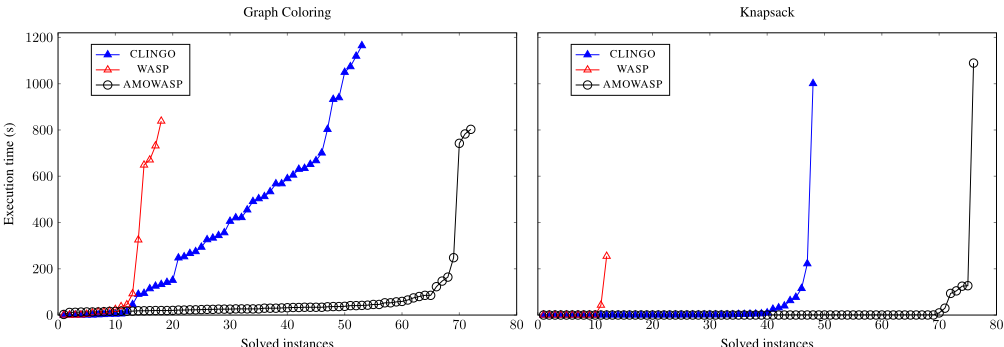
Figure 2: Number of solved instances (x-axis) within a time limit (y-axis) for Graph Coloring (left) and Knapsack (right).

4.2 Results

The experimental results for SB are summarized in Figure 1. We can see that when part size is 10 or 100, CLINGO can handle the first three instances in an efficient way, solving them with only a few conflicts. However, this is not true when part size is 1000. This suggests that the way in which CLINGO makes decisions (branching heuristic) works better for instances with SUM aggregates of small to medium size. Moreover, as we expected, the number of conflicts is related to the bound. Specifically, instances with the smallest and largest bounds have fewer conflicts. This happens because these instances are either not constrained enough or overly constrained.

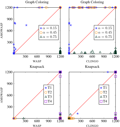
The results obtained for GC and K are summarized in Figures 2-3. As a first observation, CLINGO proves to be more efficient than WASP in both benchmarks. As highlighted in SB, the branching heuristic of CLINGO is more effective than the one of WASP. However, the inferences made by AMOWASP completely fulfil the gap related to the heuristic, and, in fact, AMOWASP achieves the best performance. Regarding GC, AMOWASP successfully solves 72 instances, surpassing CLINGO and WASP, which solve 53 and 18 instances, respectively. We additionally observe that the advantage of AMOWASP is particularly evident in instances with α = 0.75, where it outperforms CLINGO and WASP by solving 48 and 60 more instances, respectively. However, for α = 0.15 and α = 0.45, the Python implementation introduces overhead, leading to comparatively poorer performance. As for K, AMOWASP successfully solves 76 instances, outperforming both CLINGO and WASP, which solve 48 and 12 instances, respectively. We additionally observe that AMOWASP consistently outperforms WASP across all instance categories, solving 17, 25, 13, and 9 more instances of categories T1, T2, T3, and T4, respectively. In comparison to CLINGO, AMOWASP exhibits slightly poorer performance on T1 instances, where CLINGO solves one more instance. However, it demonstrates better performance on the other instances, solving 16, 4, and 9 more T2, T3 and T4 instances, respectively.

To sum up, AMOWASP outperforms WASP thanks to the technique presented in this paper, as AMOWASP is powered by WASP and thus inherits all of its heuristic parameters.

5 RelatedWork

In this work, AMOSUM constraints have been added to the (propositional) language of ASP. Nonetheless, AMOSUMs can be added to any logic-based formalism extending propositional logic, such as SMT [Nieuwenhuis et al., 2006] and CSP [Brailsford et al., 1999]. From a computational point of view, there are two main approaches to extend the capabilities of logic-based languages, namely propagator-based and translation-based, discussed below.

Solvers adopting the propagator-based approach implement ad-hoc algorithms for extending assignments with literals that are required to be true (Section 2.3). The way AMOSUM constraints are handled in this work (Section 3.2) belongs to this category. Regarding the literature, the stateof-the-art system CLINGO [Gebser et al., 2019] implements a hybrid approach for handling programs with aggregates [Gebser et al., 2009]: aggregates comprising a limited number of literals are transformed into regular rules, according to some translation-based approach, and the threshold for the number of literals is adjustable through the commandline interface; other aggregates, including the ones representing AMO constraints, are instead handled by the propagator described in Section 2.3. A similar approach is implemented also in IDP [Denecker and De Cat, 2010; Bogaerts et al., 2016] and WASP [Alviano et al., 2018]. Moreover, CLINGO and WASP offer external interfaces based on Python to define custom propagators [Cabalar et al., 2023; Dodaro and Ricca, 2020]. The propagator defined in Section 3.2 is powered by the Python interface of WASP.

Translation-based approaches consist of compilations of aggregates into alternative constructs. In the context of ASP, the similarities between aggregates and pseudo-Boolean constraints led to the adoption of some compilations of pseudoBoolean constraints into clauses [Aavani et al., 2013]. These approaches include adder circuits and binary decision diagrams [Ab´ıo et al., 2012; E´en and S¨orensson, 2006], sorting networks and watchdogs [Bailleux et al., 2009]. Regarding ASP solvers, many of these translations are incorporated into LP2SAT and LP2NORMAL [Bomanson et al., 2014; Bomanson and Janhunen, 2013], where the first solver generates CNF formulas, while the second produces normal rules. Another translation-based approach is implemented in CMODELS [Lierler and Maratea, 2004; Giunchiglia et al., 2006; Giunchiglia et al., 2008], which maps aggregates to nested logic programs [Ferraris and Lifschitz, 2005]. Finally, in the specific case of AMO constraints, translation-based approaches offer various encoding options, such as pairwise (binomial), binary (bitwise), commander, product, sequential counter, and bimander encodings (the reader is referred to [Nguyen et al., 2020] for a recent comparison of these encodings). We remark here that the AMOSUM propagator introduced in this article can be combined with AMO constraint compilers, essentially by replacing the first inference rule defined in Section 3.2 with the compiled clauses.

6 Conclusion

AMOSUM constraints extend the language of ASP with a construct designed to empower search space pruning capabilities of solvers, rather than the expressive power of the language. In fact, the construct compactly represents groups of constraints that are available in ASP with the aim of combining their knowledge to detect more deterministic consequences than those identified individually by the grouped constraints. The empirical assessment of our implementation of AMOSUM constraints confirms that their usage can provide sensible performance gains.

There are several lines of future research. First of all, AMOSUM constraints replace specific kind of constraints, precisely one SUM constraint with target bound and several at-most-one constraints, and therefore it will be interesting to search for other kinds of constraints suitable for a combined propagator. Moreover, SUM constraints are usually normalized to have a target bound, for example by flipping polarities of literals and adjusting numbers in case the constraint imposes to not exceed a given bound. Such a normalization is unnatural for AMOSUM, as flipping polarities of literals essentially breaks the AMO constraints (AMO{ℓ1, . . . , ℓn} does not imply AMO{ℓ1, . . . , ℓn}); essentially, the normalization of a constraint of the form AMOSUM{w1 : ℓ1 [s1]; · · · ; wn : ℓn [sn]} ≤ b would result into a SUM constraint. Another interesting research line is therefore the generalization of the construct introduced in this article to accommodate such transformations. In addition, AMOSUM constraints might improve the performance of existing encodings, especially in the context of scheduling [Dodaro and Maratea, 2017].

Finally, we remark here that all the material required to replicate the experiments are available at https://zenodo.org/ records/11115982 [Alviano et al., 2024].

Acknowledgments

This work was partially supported by Italian Ministry of University and Research (MUR) under PRIN project PRODE "Probabilistic declarative process mining", CUP H53D23003420006 under PNRR project FAIR "Future AI Research", CUP H23C22000860006, under PNRR project Tech4You "Technologies for climate change adaptation and quality of life improvement", CUP H23C22000370006, and under PNRR project SERICS "SEcurity and RIghts in the CyberSpace", CUP H73C22000880001; by Italian Ministry of Health (MSAL) under POS projects CAL.HUB.RIA (CUP H53C22000800006) and RADIOAMICA (CUP H53C22000650006); by Italian Ministry of Enterprises and Made in Italy under project STROKE 5.0 (CUP B29J23000430005); and by the LAIA lab (part of the SILA labs). Mario Alviano and Carmine Dodaro are members of the Gruppo Nazionale Calcolo Scientifico-Istituto Nazionale di Alta Matematica (GNCS-INdAM).