Equilibria in Two-Stage Facility Location with Atomic Clients

1 Introduction

In classical facility location [Cornu´ejols et al., 1983; Korte and Vygen, 2006], a central authority places facilities in some underlying space to serve a set of clients optimally. While this might be realistic for applications like the construction of public hospitals, in many other domains facilities are placed by selfish agents competing for clients' attention. For example, supermarkets, pubs, or fast food restaurants aim to maximize profits by trying to attract nearby clients.

Beginning with the seminal model by Hotelling [1929] and Downs [1957] in which facilities compete for clients on a line and clients always patronize their closest facility, many variants of competitive facility location models have been investigated, see [Eiselt et al., 1993; ReVelle and Eiselt, 2005; Brenner, 2011] for an overview. However, a notable feature of most competitive facility location models is that clients do not influence each other, i.e., their behavior only depends on the location of the facilities but not on the behavior of the other clients. Thus, facility agents face strategic decisions but the clients do not.

∗A full version is available at http://arxiv.org/abs/2403.03114.

In contrast to these one-sided variants, recently twosided versions featuring a client subgame have been introduced [Krogmann et al., 2021; Krogmann et al., 2023], making it a sequential two-stage game. In the first stage, the facility agents simultaneously select a location for their facilities, while in the second stage, the clients simultaneously select which facilities to patronize. In these models, the clients do interact with each other, because the client weight at a facility influences the waiting time which is the cost that the clients aim to minimize. In the previously studied models, clients are non-atomic, so they may distribute their weight among multiple facilities. The induced client subgame is a non-atomic congestion game with an essentially unique client Nash equilibrium for any given facility placement. This yields a twostage facility location game where the facilities can perfectly predict the behavior of the clients. As a consequence, subgame perfect equilibria, the suitable solution concept for sequential games, are comparatively easy to reason about.

We take this line of work to the next level by considering atomic clients, which cannot split their weights among multiple facilities. However, clients are allowed to play mixed strategies, meaning that they can randomize over which facility to patronize. Given a facility placement, the induced client subgame is then still a well-studied game, namely a singleton congestion game [Rosenthal, 1973; Fotakis et al., 2009]. Arguably, this setting is more realistic in many scenarios, like supermarket shopping or restaurant visits. The reason is that clients, conditioned on selecting one specific facility, contribute with their full weight to the congestion of the chosen facility. For example, a mixed strategy of an atomic client could represent selecting different facilities on different days.

Besides capturing a wide range of realistic facility location settings, a consequence of introducing atomic clients is the existence of multiple, potentially different Nash equilibria in the client subgame for a given facility placement. These different equilibria may also yield different congestion at facilities, so the client behavior is harder to predict for the facility agents. As a consequence, the two-stage game considered in this paper requires more involved techniques for reasoning about subgame perfect equilibria and their existence.

We develop such techniques to analyze this arguably more complex two-stage competitive facility location setting and we believe that our approach will prove versatile for understanding other multi-stage models as well. One key technique is a novel potential argument that exploits the two-staged nature of our model and the multiplicity of equilibria in the second stage. In particular, we use a hierarchical classification of the clients and sophisticated rounding in each step. This ensures that for any improving strategy change by a facility, we can carefully select a new suitable client equilibrium to sustain this improvement in the potential function value.

1.1 Model and Preliminaries

The Basics. We consider the two-stage facility location game with atomic clients, atomic 2-FLG for short, where a set of k facility agents F and a set of n client agents V interact on a given vertex-weighted directed host graph H = (V, E, w), with weight function w : V → Q+ that assigns every vertex a positive rational weight. In Section 3, we consider all clients v to be unweighted, i.e., w(v) = 1. We let the total weight of the vertices in X ⊆ V be w(X) := ∑v∈X w(v).

The vertices of H correspond to the client agents but at the same time, they also serve as possible locations for the facility agents. The weight of a vertex can be understood as the purchasing power or expected revenue of the corresponding client agent or location. Every facility agent f ∈ F can choose to locate her facility at a vertex v ∈ V , however for facility agent f, the feasible vertices may be restricted to U(f) ⊆ V . By U : F → 2V we denote the function that maps facility agents to feasible vertices. Thus, an instance of the atomic 2-FLG is specified by the triple (H,U, k). If U(f) = V for every facility agent f then we say that the instance is unrestricted and we will omit U in this case.

The Sequential Game. The atomic 2-FLG consists of two stages. First, each facility agent f selects a location sf ∈ U(f) ⊆ V for opening a facility on host graph H. Let s = (s1, . . . , sk) denote the vector of chosen facility locations for some ordering of the facility agents. Note that sf = sg is possible for different facilities f, g ∈ F. We say that s is the facility placement profile (FPP). Moreover, let S ∈ V k denote the set of all possible FPPs. In the second stage, given a FPP, each client agent v ∈ V strategically decides which facility to patronize. A client agent v can only patronize a facility f that is located in her neighborhood N(v) = {v} ∪ {u | (v, u) ∈ E}, so if sf ∈ N(v). Let Ns(v) = {f ∈ F | sf ∈ N(v)} denote the set of facilities that client v can potentially patronize, for a given FPP s. Conversely, we define the attraction range of a facility f to be As(f) = {v ∈ V | f ∈ Ns(v)}. We overload this function for a set of facilities X ⊆ F, i.e., As(X) = ⋃f∈X As(f), and Ns(X) = ⋃v∈X Ns(v), for a set of clients X ⊆ V .

A main distinguishing feature of this work is that we consider atomic clients. That means that a client v ∈ V , when patronizing a facility f ∈ Ns(v), uses her full purchasing power w(v) exclusively on facility f. However, client agents can play mixed strategies, i.e., client agents are allowed to randomize which facilities to visit.

Feasible Client Strategies. For a given FPP s, we will denote by σ(s) a client profile. The strategy of a client v ∈ V is σ(s)v, which is a probability distribution on Ns(v), the set of facilities that client v can patronize. By σ(s)v,f ∈ [0, 1] we denote the probability that client v patronizes facility f ∈ Ns(v). For given s, no facility might be available for some clients v, i.e., Ns(v) = ∅. In this case, such clients do not patronize any facility. We therefore define a strategy profile, for given FPP s, as a function σ(s) : V → [0, 1]k that has to fulfill the feasibility conditions: For each client v ∈ V ,

Since we have a sequential game with two stages, the strategy of the client agents must be specified for all possible FPPs s. Thus, the full client profile is defined by a function σ : S × V → [0, 1]k . Such a full client profile σ is feasible if σ(s) is feasible for every s ∈ S. Moreover, let Σ denote the set of all feasible full client profiles and let Σs denote the set of all feasible client profiles for a given FPP s.

Objectives. An outcome of the atomic 2-FLG on a given host graph H is defined by the tuple (s, σ), where s ∈ S and σ ∈ Σ. Any outcome entails expected facility loads, where the expected facility load of facility f in outcome (s, σ) is

Thus, ℓf(s, σ) captures the expected demand that is realized at facility f under client behavior σ. Naturally, we assume that facility agents seek a facility placement to maximize this expected demand. From the viewpoint of the clients, however, the expected facility loads are seen as congestion, i.e., as waiting time at the given facility. We assume that clients want to minimize their expected waiting time Lv(s, σ), being

where ℓ-v,f (s, σ) = ∑u̸=v σ(s)u,f · w(u) is the expected load of facility f contributed by all client agents other than v. We also call ℓ-v,f (s, σ) the v-excluded load of facility f.

Equilibria. For a given FPP s, we say that σ(s) is a client equilibrium, if no client v ∈ V has an alternative client strategy σ′ (s)v such that Lv(s, (σ′ (s)v, σ(s)-v)) < Lv(s, σ(s)), where, as usual, σ(s)-v denotes the strategies of all clients except v. See Figure 1 for examples.

A state (s, σ) is a subgame perfect equilibrium (SPE) if

1. σ(s′ ) is a client equilibrium for each FPP s′ and
2. for no facility f there exists a location s′f such that ℓf ((s′f , s-f ), σ) > ℓf (s, σ).

For an α-approximate SPE, we replace (2) with the following relaxation: For no facility f there exists a location s′f such that ℓf ((s′f , s-f ), σ) > α · ℓf (s, σ), for some α ≥ 1.

Social Welfare. We measure the social welfare of a facility placement profile s using the weighted participation rate w(s) = ∑v:Ns(v)̸=∅ w(v), which is the total client weight covered by at least one facility. With this, we define the price of anarchy (PoA) [Koutsoupias and Papadimitriou, 1999] as

where OPT(H,U, k) is the FPP with the highest weighted participation rate and worstSPE(H,U, k) the FPP s for the SPE (s, σ) with the lowest weighted participation rate. Observe that the PoA is only well-defined if a SPE exists with a weighted participation rate greater than 0.

1.2 RelatedWork

For one-sided competitive facility location, the HotellingDowns model was also analyzed on graphs [P´alv¨olgyi, 2011; Fournier, 2019; Fournier and Scarsini, 2019], where the clients reside on the edges. A discrete version of this is the Voronoi game [Ahn et al., 2004; D¨urr and Nguyen, 2007], with facilities and clients placed on the nodes of an underlying network. Also, graph-based models with limited attraction range of facilities have been studied [Feldman et al., 2016; Shen and Wang, 2017; Cohen and Peleg, 2019], where clients patronize facilities only within a certain distance and split their weight equally among them. Other non-cooperative variants have been investigated, e.g., [Vetta, 2002; Cardinal and Hoefer, 2010; Sab´an and Moses, 2012].

To the best of our knowledge, the first model where the clients also face strategic decisions was proposed by Kohlberg [1983]. In this model, the clients' cost function is a linear combination of distance and waiting time. Kohlberg shows the existence of a SPE for two facilities. Later, Peters et al. [2018] extended this to four and six facilities, if the cost function is heavily tilted towards waiting time, and Feldotto et al. [2019] investigate approximate SPE.

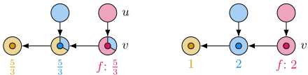
Closest to our work are the models by Krogmann et al. [2021] and Krogmann et al. [2023]. They consider nonatomic clients that split their weights among nearby facilities to either minimize (1) their maximum waiting time or (2) their total waiting time. While for (1) SPE exist, for (2) deciding SPE existence is NP-hard but approximate SPE can be computed efficiently. In contrast to both variants, we consider clients who cannot split their weight among multiple facilities. However, clients may use randomized strategies. This subtle difference is important since it yields different equilibria, i.e., randomizing over atomic strategies is not the same as non-atomic weight splitting, see Figure 2. Moreover, we also allow agent-dependent restrictions for the placement of facilities, which makes our model more general.

Besides the analysis of competitive facility location, many recent works [Kanellopoulos et al., 2022; Walsh, 2022;

Deligkas et al., 2022; Ma et al., 2023] consider a mechanism design point of view. There, clients submit their locations to a mechanism that selects positions for opening facilities. See [Chan et al., 2021] for an overview.

1.3 Our Contribution

To the best of our knowledge, the two-stage facility location game with atomic, i.e., unsplittable clients has not been considered before. It is more complex than the earlier considered two-stage facility location games with splittable clients, as client equilibria are no longer unique, and may even be qualitatively different with respect to their facility loads. We first prove the existence of subgame perfect equilibria for clients with unit weights, by using a modified best response dynamic. For clients with arbitrary weights, we show that the existence of subgame perfect equilibria is not guaranteed, and that it is even NP-complete to decide if a ϕ-approximate subgame perfect equilibrium exists, for the golden ratio ϕ ≈ 1.618. Using the utilitarian social welfare of the facilities, which equals the weighted participation rate, we also prove a tight bound of 2 on the price of anarchy, given that an equilibrium exists.

2 Client Equilibria

Given a FPP s, the client subgame is an example of the well-studied (weighted) singleton congestion game. The unweighted version has the finite improvement property and thus an improving response dynamic always converges to a pure Nash equilibrium [Rosenthal, 1973]. For the weighted version, Fotakis et al. [2009] show that pure Nash equilibria always exist and can be computed efficiently.

We first observe that in a (mixed) client equilibrium a client v only patronizes certain facilities in her shopping range.

Observation 1 (Client Patronage Set). A client profile σ(s) ∈ Σs is a client equilibrium for a given FPP s if and only if for each v ∈ V , the set of her patronized facilities {f ∈ F | σ(s)v,f > 0} contains only facilities with minimal vexcluded load within her shopping range Ns(v).

Thus, we may check in polynomial time if a client profile is a client equilibrium. Client equilibria are however not necessarily unique and might induce different facility loads.

Observation 2 (Qualitatively Different Client Equilibria). For a given facility placement profile, the number of client equilibria is not necessarily bounded and different client equilibria may induce different facility loads.

Proof. Consider an unweighted instance with a single node v and k = 2 facility agents placed on v. For every γ ∈ [0, 1], the client profile σ(s) with σ(s)v = (γ, 1 - γ) is a client equilibrium. Furthermore, the expected facility loads γ and 1 - γ differ for every value of γ.

3 Subgame Perfect Equilibria

We now prove the existence of SPE for the unweighted atomic 2-FLG via slightly modified improving response dynamics for the facility agents. We use the sorted vector of facility loads as a potential function, but after each facility move, we also select a new full client equilibrium. This is necessary because there exist improving facility moves that decrease the value of the potential function. We prevent these moves by changing to a full client equilibrium that consistently favors the facilities that already receive more load. We show that this change does not affect the value of the potential function.

3.1 Rounded Client Profiles

To determine suitable candidates for strategy profiles that yield SPE, we first partition the set of clients and the set of facilities into classes. To that end, we implicitly employ a process that repeatedly removes those facilities that have the least (average) number of clients in their range. To achieve this, we define the minimum neighborhood set 1 as the set of facilities that has the smallest average number of clients in its attraction range for a given subset of clients and facilities.

Definition 1 (Minimum Neighborhood Set (MNS)). For a facility placement profile s, a subset F ∗ ⊆ F and another subset V ∗ ⊆ V , we denote the minimum neighborhood set MNSs(F ∗ , V ∗ ) as the largest subset of F ∗ with

We now repeatedly remove a MNS and its associated set of clients from the game and assign both sets to a class.

Definition 2 (Class Set). For i ≥ 1, the class Ci = (Fi, Vi) is inductively defined by

For class Ci, denote its average load ℓ(Ci) := w(Vi) |Fi| . For a FPP s, we call C := {C1,C2, . . .} the class set of s. For a client v, let C(v) be the class of v, i.e., C(v) = Ci with v ∈ Ci. Similarly, C(f) is the class containing facility f.

An example is shown in Figure 3. We note that due to minimum neighborhood sets being of maximal cardinality, the loads of classes are pairwise different and increasing.

Corollary 1 (Uniqueness of Class Set). For an instance of the 2-FLG and the FPP s, the class set is unique. Moreover, we have ℓ(Ci) < ℓ(Ci+1) for all i ≥ 1.

Since a client is added to a class the first time one of the facilities in her shopping range is added to a class, she is in the lowest class in her neighborhood.

1 We note the difference to the definition of Krogmann et al. [2021], as we ensure uniqueness of the MNS. Furthermore, the explicit definition of Fi and Vi allows for easier recursion.

Corollary 2 (Clients in Lowest Class of Neighborhood). Each client v is in class C(v) = Cj with j = min{i | Ci ∩Ns(v) ̸= ∅}.

Krogmann et al. [2021] give an algorithm to compute a MNS 2 which we use repeatedly to compute the class set.

Corollary 3 (Class Set Computation). For a FPP s, the class set and the average loads may be computed efficiently.

We now introduce rounded client profiles which we obtain by assigning the clients to facilities within each class Ci. Note, that the definition only allows pure client strategies.

Definition 3 (Rounded Client Profile). For a FPP s, a client profile σ(s) is called rounded if for all fj ∈ F it holds that

and that each client is assigned to exactly one facility in her class. That is, for each v ∈ Vi there is exactly one f ∈ Fi with σ(s)v,f = 1. We call a full client profile σ rounded if σ(s) is rounded for each s ∈ S.

We observe that every rounded client profile is stable.

Lemma 1. A rounded client profile is a client equilibrium.

Proof. Assume for the sake of contradiction that σ(s) is not a client equilibrium. Hence, there exists some client v that is assigned to facility f, and there is another facility g ∈ Ns(v) with ℓg(s, σ) + 1 < ℓf (s, σ). Let Ci be the class of v and f . Since ℓg(s, σ) + 1 < ℓf (s, σ), facility g has to be in a class Cj with j < i and ℓ(Cj) < ℓ(Ci). However, by definition of the class sets, v should have been assigned to class Cj and not Ci, which yields the contradiction.

We now establish the existence of a rounding scheme that yields rounded client profiles, thereby proving their existence. In particular, this implies that pure client equilibria exist.

Theorem 1 (Existence of Rounded Profiles). For every unweighted instance of the atomic 2-FLG and facility placement profile s, there exists a rounded client profile σ(s).

Proof. We compute a rounded client profile by appropriately assigning the clients to facilities for each class separately:

For each class Ci, we define the directed, bipartite residual graph Ri based on a current (pure) client profile σ(s). Let Ri = (Vi ∪ Fi, Ei) with (f, v) ∈ Ei if σ(s)v,f = 0 and v ∈ As(f), and the reverse edge in (v, f) ∈ Ei if σ(s)v,f = 1. We start with all clients unassigned and repeat the following steps until all clients of Ci are assigned:

1. Let F ∗ ⊆ Fi be the facilities of Ci with lowest current load.

2 We show in the full version [Krogmann et al., 2024], why their algorithm is applicable despite the different definitions.

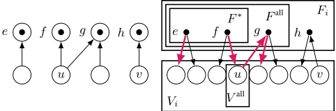
1. In the residual graph Ri, find a simple path from set F ∗ to the set of unassigned clients in Vi, i.e., the result is a path between some facility of current minimal load and some unassigned client.
2. Use the path to augment the client assignment, i.e, if there is an edge (f, v) in the path, then assign v to f and if there is an edge (v, f), then unassign v from f.

Figure 4 shows an intermediate state of an example run of this procedure. Step 3 keeps the facility loads constant for all facilities except for the first one in the path. By the choice of F ∗ , we maintain the invariant that the maximum difference of facility loads is 1. Hence in the end the loads must be ⌊ℓ(Ci)⌋ or ⌈ℓ(Ci)⌉ and the result is a rounded client equilibrium.

It remains to show that the path in Step 2 always exists in each iteration. Assume towards contradiction that there is no such path, but an unassigned client. Let F all be the set of all facilities reachable from the set F ∗ (with F ∗ ⊆ F all ) and let V all be the set of clients currently assigned to any facility in F all . We have V all = As(F all ) ∩ Vi as there is no unassigned client reachable from F ∗ and any assigned client in As(F all ) ∩ Vi has an edge to her assigned facility, meaning that her facility is also in F all . Now Fi \F all ̸= ∅, because the unassigned client is in the attraction range of some facility in Fi. Since all facilities in Fi \ F all have a load higher than the average of F all , we get

which contradicts Fi being a minimum neighborhood set.

We later use the lexicographic increasingly sorted vector of facility loads ℓsort as a potential function. By construction of the class set and by definition of rounded client profiles, we immediately get the following.

Observation 3 (Identical Load Vector for Rounded Profiles). For an instance of the unweighted atomic 2-FLG and a facility placement profile s, let σ(s) and σ′ (s) denote two rounded client profiles for s. Then, ℓsort(s, σ) = ℓsort(s, σ′ ).

This enables switching between distinct rounded client equilibria without changing the potential function ℓsort.

3.2 Favoring Client Equilibria

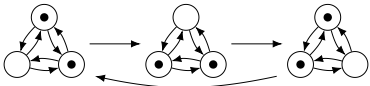
We later seek to find a SPE by means of a sequence of improving facility moves. However, it turns out, that it is not sufficient to do so with an arbitrary (rounded) full client equilibrium. Due to differences in the rounding in σ for different FPPs s, there might exist an improvement sequence that cycles through a sequence of FPPs s1, s2, . . . , sm, s1, while ℓsort(si, σ) = ℓsort(sj , σ) for all i, j. See Figure 5.

To circumvent cycling, we need to ensure that rounding is consistent between FPPs. We solve that by making sure that the clients favor facilities based on a specifically chosen ordering of the facilities. Therefore, for a given permutation π of the set of facilities, let us first define a π-favoring rounded equilibrium as follows.

Definition 4 (π-favoring). For a fixed permutation π of the set of facilities, let ℓπ := (ℓπ(1)(s, σ), . . . , ℓπ(k)(s, σ)). A rounded client equilibrium σ(s) is π-favoring if it maximizes the vector ℓπ lexicographically among all rounded client profiles for s. Similarly, a full client equilibrium σ is π-favoring if σ(s′ ) is a π-favoring client equilibrium for every s′ ∈ S.

As our key technical ingredient, we next show that any improving facility move from (s, σ) increases the vector ℓsort lexicographically if σ is π-favoring for a specific permutation π. In particular, for this π the entries of ℓπ are non-increasing.

Lemma 2 (Lexicographical Potential Increase). Let s be a facility placement profile. Every improving facility move away from (s, σ) strictly increases ℓsort lexicographically if σ is πfavoring for a permutation π with the following property: For all f, g ∈ F , if ℓf (s, σ) > ℓg(s, σ), then π-1 (f) < π-1 (g).

Proof. Assume for the sake of contradiction that some facility f can improve, changing the state from s to s′ but without increasing ℓsort lexicographically. Let C = {C1, C2, . . .} and C ′ = {C ′1 , C ′2 , . . .} be the class sets for s and s′ , respectively. Since the load of f increased but ℓsort did not increase lexicographically, there exists a facility d ∈ F with

As σ is a rounded full client profile, by Definition 3, we have

For our analysis, we construct the following reassignment graph G that captures the difference in client assignment between σ(s) and σ(s′ ). This is a directed, multigraph G = (F,E) where we add an edge (f1, f2) for every v with σ(s)v,f1 = 1 and σ(s′ )v,f2 = 1. As the load of d has decreased, the out-degree of d is strictly larger than her indegree in G. Therefore, there exists a directed path p from d to a facility g which has an in-degree that is strictly larger than her out-degree. Comparing the assignments of the clients that determine the edges of p between σ(s) and σ(s′ ), we observe that the difference only affects the loads of d and g. Hence for this facility g, we have

Again, by Definition 3, we have

For any two consecutive facilities a, b on the path p, there is a client v that is assigned to a in s and b in s′ . By Corollary 2 we conclude that ℓa(s, σ) ≤ ℓb(s, σ) and ℓa(s′ , σ) ≥ ℓb(s′ , σ). This implies for the average load of the respective classes ℓ(C(a)) ≤ ℓ(C(b)) and ℓ(C ′ (a)) ≥ ℓ(C ′ (b)) which yields

We now distinguish two cases.

Case 1: g ̸= f. Combining (4) with (2) and (5) results in

And, hence, the above holds with equality. By (1), (3), and Definition 3, we get that

By (6) and (7), we have that both assignments of the clients that determine the path p yield a feasible rounded client equilibrium for both s and s′ . As d is preferred in σ(s), we must have π-1 (d) > π-1 (g), however, from σ(s′ ), we get that π-1 (g) > π-1 (d), which yields the contradiction.

Case 2: g = f. Using (5), Definition 3, and (1) we have

By f improving from s to s′ and Definition 3:

which implies equality for

Together with (1) we get ℓd(s, σ) > ℓf(s, σ) which implies π-1 (d) < π-1 (f) by the additional property of the lemma. This, however, contradicts σ(s′ ) being π-favoring. In σ(s′ ), assigning the clients that determine path p as in σ(s) lexicographically increases ℓπ since the load of d increases by 1 while the load of f decreases by 1.

Observe that this still yields a feasible rounded client profile as the loads of all facilities except d and f did not change and we have that ℓf (s′ , σ) = ⌊ℓ(C ′ (f))⌋ + 1 and since ℓ(C ′ (d)) ≥ ℓ(C ′ (f)) and ⌊ℓ(C ′ (d))⌋ = ℓd(s′ , σ) also ℓd(s′ , σ) + 1 = ⌈ℓ(C ′ (d))⌉.

In both cases we reached a contradiction, hence such a facility d cannot exist. The lemma follows.

The existence of π-favoring client equilibria and πfavoring full client equilibria follows directly from Theorem 1 and Definition 4. Moreover, we show that a π-favoring full

Algorithm 1: findFavoringEquilibrium(H, s, π)

• 1 G ← (F ∪ V ∪ {s, t}, EN ∪ Es ∪ Et ∪ Eadd);
• 2 Es ← {(s, v, 1, 0) | v ∈ V };
• 3 EN ← {(v, f, 1, 0) | C(v) = C(f) ∧ f ∈ Ns(v)};
• 4 Et ← {(f, t, ⌊ℓ(C(f))⌋, 2k ) | f ∈ F};
• 5 Eadd ← {(f, t, 1, 2k-π-1 (f) ) | f ∈ F};
• 6 compute integral s-t-MAXCOSTFLOW on G;
• 7 for v ∈ V do
• 8 assign v to facility f with nonzero flow on (v, f);

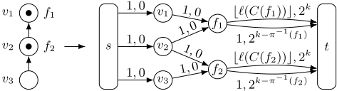
client equilibrium can be computed in polynomial time. Algorithm 1 computes π-favoring client equilibria by employing a reduction to integral MAXCOSTFLOW, where for each client a demand of 1 flows to the facilities of her class in her shopping range and then to a sink node t.

Figure 6 shows an example of the construction. Each facility f has one edge with capacity ⌊ℓ(C(f))⌋ and cost 2k to t and a second edge to t with capacity 1 and cost 2k-π-1 (f) . This ensures that each facility receives an allowed value of load for a rounded client equilibrium, while the cost of the edges with capacity 1 prefers facilities appearing earlier in π.

Theorem2 (π-favoring Equilibria Complexity). For any FPP s and any π, a π-favoring client equilibrium σ can be computed in polynomial time.

A detailed proof is in the full version [Krogmann et al., 2024].

3.3 Constructing a Subgame Perfect Equilibrium

We now prove the existence of SPEs by providing an algorithm that computes one. We start with an arbitrary FPP s and full client profile σ. If (s, σ) is not a SPE, i.e., there is a facility that can improve resulting in a profile (s′ , σ), we determine a possibly different full client profile σ′ that satisfies the conditions of Lemma 2 for a possibly different π′ . We repeat this process until we find a SPE. This process terminates as by Lemma 2 in each step the value of ℓsort increases.

Theorem 3 (Existence of SPE). Every instance of the unweighted atomic 2-FLG admits a subgame perfect equilibrium with a pure full client equilibrium.

Proof. We show that Algorithm 2 computes a SPE. By Theorem 1, an initial rounded profile σ exists. A π-favoring full client equilibrium exists by Theorem 1 and Definition 4. It remains to show that this algorithm terminates. To that end, we show that in each iteration except the first, the vector of sorted facility loads increases lexicographically.

Algorithm 2: findSPE(H, U, k)

1 s ←arbitrary facility placement profile;

2 σ ← arbitrary rounded full client profile; 3 while (s, σ) is not a SPE do 4 s ← execute arbitrary improving facility move; 5 π ← facilities sorted by decreasing loads in σ(s); 6 σ ←a π-favoring full client equilibrium;

The conditions of Lemma 2 are satisfied by the permutation π in Line 5, so for every improving facility move in Line 4 with the facility placement profiles s and s′ before and after the move, the value of ℓsort lexicographically increases:

By Observation 3, ℓsort does not change when switching to a different rounded full client equilibrium in Line 6 while keeping the FFP s fixed. Since the number of possible facility placement profiles is finite, the algorithm terminates.

Regarding the complexity of computing a SPE, we note that a full client equilibrium requires exponential space because there are exponentially many FPPs for which clients need to specify a client profile. However, for certifying the existence of a SPE and for Algorithm 2, it is sufficient to specify the client equilibria for the chosen state s and all states s′ with only a single facility deviation. With that caveat, each iteration of Algorithm 2 can be performed in polynomial time. However, the number of iterations needed is an open problem.

4 SPE in theWeighted Game

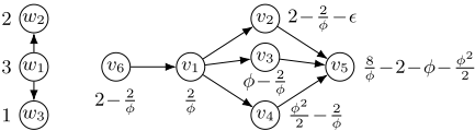
We now turn to instances with weighted clients. Here, SPE do not exist in all instances and it is even NP-complete to decide whether an approximate SPE exists that has a ratio smaller than the golden ratio ϕ. In Figure 7, we show a simple instance with no SPE and another one that does not admit a (ϕ - ϵ)-approximate SPE. In the full version [Krogmann et al., 2024], we give detailed proof of the non-existence.

Theorem 4 (Nonexistence of Weighted SPE). Weighted instances of the atomic 2-FLG might not admit SPE.

Theorem 5 (Approximate Weighted SPE Lower Bound). Weighted instances of the atomic 2-FLG might not admit (ϕ - ϵ)-approximate SPE for any ϵ > 0.

It is open if this bound is tight. Note that a k-approximate SPE always exists: Place each facility on the single vertex with the highest total client weight in her attraction range, and let the clients use equal probabilities for each facility.

Observation 4 (Approximate SPE Upper Bound). Each instance of the 2-FLG admits a k-approximate SPE.

We can even show that deciding whether a (ϕ - ϵ)- approximate SPE exists is NP-complete via a reduction from SAT. Membership in NP is given by the fact that a FPP and client equilibria for only the polynomially many neighboring FPPs are sufficient to verify the existence of a SPE. We give detailed proof in the full version [Krogmann et al., 2024].

Theorem 6 (Complexity of Approximate Weighted SPE). Let α ∈ [1, ϕ) denote some multiplicative approximation ratio. It is NP-complete to decide whether a weighted instance of the atomic 2-FLG admits an α-approximate SPE.

5 EquilibriumEfficiency

Note that the weighted participation rate captures both the social welfare of the clients and the facilities. Note that for the clients the waiting time is not taken into account, only whether they are served at all. We prove that the PoA is exactly 2. This improves the upper bound of Krogmann et al. [2021] that only holds for instances where each facility may choose any location. Also, as another contrast, in the full version [Krogmann et al., 2024] we show a matching lower bound. There, we also show how to transfer their lower bound of 2 - 1k on the price of stability to our model.

Theorem 7 (Price of Anarchy). For the weighted atomic 2FLG, the price of anarchy regarding the utilitarian social welfare of the facility agents is 2 for k ≥ 2 facility agents.

Proofsketch. We consider an instance (H,U, k) of 2-FLG with k ≥ 2, and let (s, σ) denote some SPE. Let V un (s) denote the set of uncovered clients with no facility in their shopping range for s. We say a subset V ′ ⊆ V un (s) is an f-cluster if they can all be covered by facility f at the same time, i.e., if there exists a vertex v ∈ U(f) such that V ′ ⊆ N(v). Since s is a facility equilibrium, the maximum weight of an f-cluster is ℓf (s, σ), as otherwise, f could improve by at least the complete weight of the f-cluster by moving to v.

For each f ∈ F, let V f denote an f-cluster of maximal weight. Then the total weight of clients in V un (s) covered by an alternative FPP is at most ∑f∈F w(V f ). Any such alternative FPP may still cover all previously covered clients, so we bound W(OPT) as follows: W(OPT) ≤

Therefore, the price of anarchy is at most 2.

6 Conclusion

Even though two-stage facility location games with atomic clients may have qualitatively distinct client equilibria, we demonstrate that SPE exist for the case of unweighted clients, and that this no longer holds for non-uniform clients. Our proof of existence via modified best response dynamics introduces several novel ideas that may be useful also beyond facility location. For the weighted case, the conjecture that ϕapproximate SPE always exist, remains an open problem. We believe our work serves as a starting point for further research into more complex competitive facility location models.

Acknowledgements

This work was supported by the Federal Ministry of Education and Research (BMBF) with a fellowship within the IFI program of the German Academic Exchange Service (DAAD).