
Two Influence Maximization Games on Graphs Made Temporal
Proceedings of the Thirtieth International Joint Conference on Artificial Intelligence. Main Track. Pages 45-51.
https://doi.org/10.24963/ijcai.2021/7
Keywords
- Agent-based and Multi-agent Systems: Noncooperative Games
- Agent-based and Multi-agent Systems: Algorithmic Game Theory
Abstract
To address the dynamic nature of real-world networks, we generalize competitive diffusion games and Voronoi games from static to temporal graphs, where edges may appear or disappear over time. This establishes a new direction of studies in the area of graph games, motivated by applications such as influence spreading. As a first step, we investigate the existence of Nash equilibria in competitive diffusion and Voronoi games on different temporal graph classes. Even when restricting our studies to temporal paths and cycles, this turns out to be a challenging undertaking, revealing significant differences between the two games in the temporal setting. Notably, both games are equivalent on static paths and cycles. Our two main technical results are (algorithmic) proofs for the existence of Nash equilibria in temporal competitive diffusion and temporal Voronoi games when the edges are restricted not to disappear over time.
- [Ahn et al., 2004] Hee-Kap Ahn, Siu-Wing Cheng, Otfried Cheong, Mordecai J. Golin, and René van Oostrum. Com- petitive facility location: the Voronoi game. Theor. Com- put. Sci., 310(1-3):457-467, 2004.
- [Alon et al., 2010] Noga Alon, Michal Feldman, Ariel D Procaccia, and Moshe Tennenholtz. A note on competi- tive diffusion through social networks. Inf. Process. Lett., 110(6):221-225, 2010.
- [Bandyapadhyay et al., 2015] Sayan Bandyapadhyay, Aritra Banik, Sandip Das, and Hirak Sarkar. Voronoi game on graphs. Theor. Comput. Sci., 562:270-282, 2015.
- [Banik et al., 2013] Aritra Banik, Bhaswar B. Bhattacharya, and Sandip Das. Optimal strategies for the one-round dis- crete Voronoi game on a line. J. Comb. Optim., 26(4):655- 669, 2013.
- [Bentert et al., 2020] Matthias Bentert, Anne-Sophie Him- mel, André Nichterlein, and Rolf Niedermeier. Efficient computation of optimal temporal walks under waiting- time constraints. Appl. Netw. Sci., 5(1):73, 2020.
- [Bulteau et al., 2016] Laurent Bulteau, Vincent Froese, and Nimrod Talmon. Multi-player diffusion games on graph classes. Internet Math., 12(6):363-380, 2016.
- [Chauhan et al., 2018] Ankit Chauhan, Pascal Lenzner, and Louise Molitor. Schelling segregation with strategic agents. In Proc. of SAGT '18, pages 137-149. Springer, 2018.
- [Cheong et al., 2004] Otfried Cheong, Sariel Har-Peled, Nathan Linial, and Jiří Matoušek. The one-round Voronoi game. Discrete Comput. Geom., 31(1):125-138, 2004.
- [de Berg et al., 2019] Mark de Berg, Sándor Kisfaludi-Bak, and Mehran Mehr. On one-round discrete Voronoi games. In Proc. of ISAAC '19, pages 37:1-37:17. Schloss Dagstuhl -Leibniz-Zentrum für Informatik, 2019.
- [Dürr and Thang, 2007] Christoph Dürr and Nguyen Kim Thang. Nash equilibria in Voronoi games on graphs. In Proc. of ESA '07, pages 17-28. Springer, 2007.
- [Echzell et al., 2020] Hagen Echzell, Tobias Friedrich, Pas- cal Lenzner, and Anna Melnichenko. Flow-based network creation games. In Proc. of IJCAI '20, pages 139-145. IJCAI
- [Elkind et al., 2019] Edith Elkind, Jiarui Gan, Ayumi Igarashi, Warut Suksompong, and Alexandros A. Voudouris. Schelling games on graphs. In Proc. of IJCAI '19, pages 266-272. ijcai.org, 2019.
- [Erlebach and Spooner, 2020] Thomas Erlebach and Jakob T. Spooner. A game of cops and robbers on graphs with periodic edge-connectivity. In Proc. of SOFSEM '20, pages 64-75. Springer, 2020.
- [Etesami and Bas ¸ar, 2016] Seyed Rasoul Etesami and Tamer Bas ¸ar. Complexity of equilibrium in competitive diffusion games on social networks. Automatica, 68:100-110, 2016.
- [Fekete and Meijer, 2005] Sándor P. Fekete and Henk Mei- jer. The one-round Voronoi game replayed. Comput. Geom., 30(2):81-94, 2005.
- [Feldmann et al., 2009] Rainer Feldmann, Marios Mavroni- colas, and Burkhard Monien. Nash equilibria for Voronoi games on transitive graphs. In Proc. of WINE '09, pages 280-291. Springer, 2009.
- [Fukuzono et al., 2020] Naoka Fukuzono, Tesshu Hanaka, Hironori Kiya, Hirotaka Ono, and Ryogo Yamaguchi. Two-player competitive diffusion game: Graph classes and the existence of a Nash equilibrium. In Proc. of SOF- SEM '20, pages 627-635. Springer, 2020.
- [Ito et al., 2015] Takehiro Ito, Yota Otachi, Toshiki Saitoh, Hisayuki Satoh, Akira Suzuki, Kei Uchizawa, Ryuhei Ue- hara, Katsuhisa Yamanaka, and Xiao Zhou. Competitive diffusion on weighted graphs. In Proc. of WADS '15, pages 422-433. Springer, 2015.
- [Kumabe and Maehara, 2020] Soh Kumabe and Takanori Maehara. Convexity of b-matching games. In Proc. of IJCAI '20, pages 261-267. ijcai.org, 2020. IJCAI
- [Mavronicolas et al., 2008] Marios Mavronicolas, Burkhard Monien, Vicky G. Papadopoulou, and Florian Schopp- mann. Voronoi games on cycle graphs. In Proc. of MFCS '08, pages 503-514. Springer, 2008.
- [Morawietz and Wolf, 2021] Nils Morawietz and Petra Wolf. A timecop's chase around the table. CoRR, abs/2104.08616, 2021.
- [Morawietz et al., 2020] Nils Morawietz, Carolin Rehs, and Mathias Weller. A timecop's work is harder than you think. In Proc. of MFCS '20, pages 71:1-71:14. Schloss Dagstuhl -Leibniz-Zentrum für Informatik, 2020.
- [Roshanbin, 2014] Elham Roshanbin. The competitive dif- fusion game in classes of graphs. In Proc. of AAIM '14, pages 275-287. Springer, 2014.
- [Small and Mason, 2013] Lucy Small and Oliver Mason. Nash equilibria for competitive information diffusion on trees. Inf. Process. Lett., 113(7):217-219, 2013.
- [Sukenari et al., 2016] Yuki Sukenari, Kunihito Hoki, Satoshi Takahashi, and Masakazu Muramatsu. Pure Nash equilibria of competitive diffusion process on toroidal grid graphs. Discrete Appl. Math., 215:31-40, 2016.
- [Sun et al., 2020] Xiaoming Sun, Yuan Sun, Zhiyu Xia, and Jialin Zhang. The one-round multi-player discrete Voronoi game on grids and trees. Theor. Comput. Sci., 838:143- 159, 2020.
- [Takehara et al., 2012] Reiko Takehara, Masahiro Hachi- mori, and Maiko Shigeno. A comment on pure-strategy Nash equilibria in competitive diffusion games. Inf. Pro- cess. Lett., 112(3):59-60, 2012.
- [Teramoto et al., 2011] Sachio Teramoto, Erik D. Demaine, and Ryuhei Uehara. The Voronoi game on graphs and its complexity. J. Graph Algorithms Appl., 15(4):485-501, 2011.
References were extracted automatically from the PDF and may contain errors.
Full text extracted automatically from the PDF; figures, tables and equations may differ. The PDF is the version of record.
1 Introduction
As graph games help us to reason about a networked world, playing games on graphs is an intensively researched topic since decades. In this work, we focus on competitive games on undirected graphs. Here, some external parties influence a small subset of agents who then spread some information through the network. Typical application scenarios for these occur, for instance, when political parties aim to gain influence in a social network or in the context of viral marketing.
Looking at two prominent, somewhat similar representatives, namely competitive diffusion games and Voronoi games, we put forward to model network dynamics more realistically. Specifically, while to the best of our knowledge almost all work on graph games focused on static graphs, we initiate the study of these two games on temporal graphs. Roughly speaking, in a temporal graph, the edge set may evolve over discrete time steps, while the vertex set remains unchanged, yielding time-ordered graph layers with different edge sets. Moving to the temporal setting has dramatic consequences. For example, while competitive diffusion games and Voronoi games are equivalent on static paths and cycles [Sun et al., 2020] and we understand well their properties in these simple but important special cases, they are no longer equivalent in the temporal case and their properties are much more challenging to analyze.
Our study takes a first step towards understanding both games on temporal paths and cycles. It turns out that these two backbone structures of graphs already confront us with several technically challenging questions when looking for the existence (and computation) of Nash equilibria-one of the most fundamental game-theoretic concepts. We refer to the next section for formal definitions and examples of the two (temporal) games. Intuitively speaking, in both games one can think of each player having a color and trying to color as many vertices as possible by her own color; the coloring process starts in a vertex freely chosen by each player and acts through the neighborhood relation of the graph. Herein, the distance of a vertex to the start vertices plays a central role. In both games, a player colors all vertices that are closest to her start vertex. Moreover, while in competitive diffusion games a vertex that is at the same distance to two start vertices of competing players can still get one of the two colors, this is not the case for Voronoi games.
Related work. Competitive diffusion games were introduced by Alon et al. [2010]. Research on competitive diffusion games so far mainly focused on the existence of Nash equilibria on a variety of graph classes for different numbers of players [Alon et al., 2010; Bulteau et al., 2016; Fukuzono et al., 2020; Roshanbin, 2014; Small and Mason, 2013; Sukenari et al., 2016; Takehara et al., 2012]. Also, the (parameterized) computational complexity of deciding the existence of a Nash equilibrium has been studied [Etesami and Bas¸ar, 2016; Ito et al., 2015].
Voronoi games have been originally studied for a onedimensional or two-dimensional continuous space [Ahn et al., 2004; Banik et al., 2013; de Berg et al., 2019; Cheong et al., 2004; Fekete and Meijer, 2005]. There, it is typically assumed that players choose their initial sets of points sequentially and that a player wins the game if a certain fraction of all points is closest to her. Voronoi games on graphs have also been studied on different graph classes for various numbers of players [Bandyapadhyay et al., 2015; D¨urr and Thang, 2007; Feldmann et al., 2009; Mavronicolas et al., 2008; Sun et al., 2020; Teramoto et al., 2011]. Again a focus lies on determining for which graphs a Nash equilibrium exists and how to compute one.
| Superset | Monotonically growing | Monotonically shrinking | |
|---|---|---|---|
| Diffusion | |||
| Temporal Paths | 3 (Th. 2) | 3 (Th. 2) | 7 (Th. 4) |
| Temporal Cycles | 7 (Th. 5) | 3 (Th. 6) | 7 (Th. 7) |
| Voronoi | |||
| Temporal Paths | 7 (Th. 8) | 3 (Th. 9) | 7 (Co. 1) |
| Temporal Cycles | 7 (Th. 8) | ? | 7 (Co. 1) |
From a broader perspective, analyzing games played on graphs from a game-theoretic perspective is an intensively researched topic; recent examples include Schelling games [Chauhan et al., 2018; Elkind et al., 2019], b-matching games [Kumabe and Maehara, 2020], or network creation games [Echzell et al., 2020].
As mentioned before, we know of basically no work systematically studying graph games in a temporal setting. The only exception we are aware of is in the context of pursuitevasion games: Erlebach and Spooner [2020] studied the pursuit-evasion game of cops and robbers on some specific temporal graphs, namely so-called edge-periodic graphs. Also different from our studies, their focus was on computing winning strategies for the players. Morawietz et al. [2020] and Morawietz and Wolf [2021] extended this study, also answering an open question of Erlebach and Spooner [2020].
Our contributions. We put forward the study of gametheoretic models on temporal graphs. We do so by generalizing two well-studied (static) graph games to temporal graphs, namely competitive diffusion games and Voronoi games. For the two resulting temporal graph games we analyze the (constructive) existence of Nash equilibria on different temporal graph classes, focusing on different types of temporal paths and cycles (see Section 1 for an overview of our results). We observe that, in contrast to the static case where both games are equivalent and a Nash equilibrium is guaranteed to exist [Roshanbin, 2014], on temporal paths and cycles, the games exhibit far more complex dynamics and a quite different behavior. Our main results are two proofs of guaranteed existence of Nash equilibria, namely in temporal diffusion games on so-called monotonically growing temporal cycles, and in temporal Voronoi games on so-called monotonically growing temporal paths. One conclusion from our work is that temporal Voronoi games seem to be more elusive to a full understanding of fundamental properties than temporal competitive diffusion games. Correspondingly, Section 1 identifies one concrete open question for Voronoi games where we already have an answer for competitive diffusion games.
Due to lack of space, we defer several proofs (marked ⋆) to a full version available at arxiv.org/abs/2105.05987.
2 Preliminaries
For a ≤ b ∈ N, let [a, b] := {a, a+1, . . . , b}, [a, b[:= {a, a+ 1, . . . , b-1}, and ]a, b] := {a+1, . . . , b}. Further, let [n] := [1, n] for n ∈ N.
2.1 Temporal Graphs
A temporal graph is a tuple G = (V,E1, . . . ,Eτ) (or G = (V, (Ei)i∈[τ]) for short), where V is the set of vertices and E1, . . . ,Eτ a sequence of edge sets with Et ⊆ (V2 ) for t ∈ [τ]. We refer to τ as the lifetime of G. For t ∈ [τ], we call Gt = (V,Et) the t-th layer of G. Let the underlying graph of G be the graph G↓ = (V, E↓) with E↓ := ⋃t∈[τ ] Et.
A temporal path of size n (or a temporal cycle of size n) is a temporal graph G = (V, (Ei)i∈[τ]) with V = [n] such that G↓ is a path (or a cycle) of size n. For two vertices u < v ∈ [n], we say that u is left of v and v is right of u. We refer to a temporal graph G as a temporal linear forest if the connected components of G↓ are paths. Moreover, we call a temporal graph G a superset temporal graph if its last layer is identical to its underlying graph, i.e., Gτ = G↓. Further, we call G monotonically growing if no edge disappears over time, i.e., Ei ⊆ Ei+1 for all i ∈ [τ - 1]. Note that each monotonically growing temporal graph is also a superset temporal graph. Symmetrically, G is monotonically shrinking if edges do not appear over time, i.e., Ei+1 ⊆ Ei for all i ∈ [τ -1]. For the definition of temporal Voronoi games, we now introduce a notion of temporal distance of two vertices. In a temporal graph G = (V, (Ei)i∈[τ]), we define a temporal walk from a vertex v0 to a vertex vd as a sequence of tuples ({v0, v1}, t1), ({v1, v2}, t2), . . . , ({vd-1, vd}, td) such that the following properties hold:
- ti ≤ ti+1 for all i ∈ [d-1],
- {vi-1, vi} ∈ Eti for all i ∈ [d] with ti ≤ τ,
- {vi-1, vi} ∈ Eτ for all i ∈ [d] with ti > τ.
We refer to td as the arrival time of the temporal walk. Note that the last condition can be interpreted as repeating the last layer arbitrarily often. This is to allow for arrival times td > τ which is somewhat natural and closer to the static case. A temporal walk is called strict if ti < ti+1 holds for all i ∈ [d - 1]. Moreover, we call a temporal walk from v0 to vd foremost if there is no temporal walk from v0 to vd with a smaller arrival time. We now define the temporal distance td(u, v) from u to v as the arrival time of a strict foremost walk 1 from u to v. Notably, in contrast to the static case, temporal distances are not necessarily symmetric, i.e., td(u, v) ̸= td(v, u) is possible. By convention, we set td(v, v) = 0 for any vertex v. For two vertices u and v, we say that u reaches v until step ℓ if td(u, v) ≤ ℓ and that u reaches v in step (or at time) ℓ if td(u, v) = ℓ.
2.2 Games on Temporal Graphs
We focus on games with two players. Nevertheless, to highlight the nature of our definitions, we directly introduce both games for an arbitrary number of players. Since the games are somewhat similar, we start by making some general definitions for both temporal games before describing the specifics. For a temporal graph G = (V, (Ei)i∈[τ ]) and a number k ∈ N of players, Diff(G, k) (Vor(G, k)) denotes the k-player temporal diffusion game (temporal Voronoi game) on the temporal graph G, where each player has her distinct color in [k]. Moreover, we use the color 0 to which we refer as gray. The strategy space of each player i ∈ [k] is the vertex set V , i.e., each player i selects a single vertex pi ∈ V , which is then immediately colored by her color i. If two players pick the same vertex, then it is colored gray. A strategy profile of the game is a tuple (p1, . . . , pk) ∈ V k containing the initially chosen vertex of each player. We also use the term position to refer to the vertex pi chosen by player i.
1 We consider foremost walks since earliest arrival seems more natural than other concepts such as fastest or shortest [Bentert et al., 2020] in the context of influence spreading. Moreover, we consider strict temporal walks since they are closer to the static case and to the diffusion process.
Now, for both games the strategy profile (p1, . . . , pk) determines a partial coloring of the vertices in V with colors from 0, . . . , k (some vertices might remain uncolored) as described below. For a strategy profile (p1, . . . , pk), let Ui(p1, . . . , pk) be the set of vertices with color i in the resulting coloring and let ui(p1, . . . , pk) := |Ui(p1, . . . , pk)| be the number of vertices with color i. For a strategy profile (p1, . . . , pk), the payoff or outcome (of the game) of player i is ui(p1, . . . , pk). We say that a player i ∈ [k] plays a best response to the other players in the strategy profile (p1, . . . , pk) if for all vertices p′ ∈ V it holds that ui(p1, . . . , pi-1, p′ , pi+1, . . . , pk) ≤ ui(p1, . . . , pk). A strategy profile (p1, . . . , pk) is a Nash equilibrium if every player i ∈ [k] plays a best response to the other players.
It remains to specify how the strategy profile (p1, . . . pk) determines the coloring of the vertices V in the two games.
Temporal diffusion games. In a temporal diffusion game, the temporal graph G is colored by the following propagation process over time. We call a vertex uncolored if no color has been assigned to it (so far). In step t ∈ [τ], we consider the layer Gt. We color a so far uncolored vertex v with color i ∈ [k] if v has at least one neighbor in Gt that is colored with color i ∈ [k] and no neighbor in Gt that is colored with any other color j ∈ [k] \ {i}. Every uncolored vertex with at least two neighbors in Gt colored by two different colors i, j ∈ [k] is colored gray. In step t > τ, the propagation process continues on Gτ until the coloring of the vertices does not change between two consecutive steps (we again "repeat" the last layer to be consistent with the static case).
Temporal Voronoi games. In a temporal Voronoi game, a vertex v is colored with color i ∈ [k] if the arrival time of a strict foremost walk from pi to v is smaller than the respective arrival times for all other players, i.e., vertex v ∈ V is colored with color i ∈ [k] if td(pi, v) < td(pj, v) holds for all j ̸= i ∈ [k]. If at least two players have the earliest arrival time, then the vertex is colored gray.
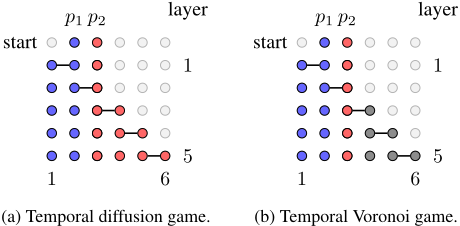
Note that we defined temporal diffusion games and temporal Voronoi games such that both temporal games played on a temporal graph G with identical layers are equivalent to the (non-temporal) game played on the static graph G↓. An example of a temporal diffusion game and a temporal Voronoi game is shown in Figure 1. Notably, in the displayed temporal diffusion game each player colors a superset of the vertices they color in the temporal Voronoi game. In fact, by definition of the two games, this holds for every temporal graph (as in the static case).
3 Temporal Diffusion Games
We start with temporal paths followed by temporal cycles.
3.1 Temporal Paths
We first prove that on a temporal path, in general, a Nash equilibrium is not guaranteed to exist, even if each edge only appears in one layer. Afterwards, we show that as soon as the temporal path fulfills the superset property, up to symmetry and tie-breaking, every game admits a unique Nash equilibrium. Lastly, we prove that enforcing that edges do not appear over time is not enough to guarantee the existence of a Nash equilibrium, even if the graph consists of only two layers.
We start by showing that the temporal diffusion game on the temporal path depicted in Figure 1 (where every edge of the underlying graph only occurs at one point of time) does not admit a Nash equilibrium. This is in contrast to the static case where a Nash equilibrium is guaranteed to exist on every path [Roshanbin, 2014, Theorem 1].
Theorem 1. There is a temporal path P such that there is no Nash equilibrium in Diff(P, 2).
Proof. We prove the theorem by showing that for P = ([6],E1, . . . ,E5) with Et = {{t, t + 1}} for t ∈ [5] (see Figure 1), there is no Nash equilibrium in Diff(P, 2). For the sake of contradiction, assume that (p1, p2) with p1 < p2 is a Nash equilibrium in Diff(P, 2). Player 1 colors all vertices in [max(1, p1 -1), p2 -1] and player 2 all vertices in [p2, n].
Note that p2 = p1 +1 must hold, as otherwise player 2 can color additional vertices by moving to vertex p1 + 1. Moreover, if p1 ≥ 3, then player 1 can additionally color vertex 1
by moving to vertex 1. Thus, p1 ∈ {1, 2}, p2 = p1 + 1, and p2 ∈ {2, 3}. However, this implies that player 1 colors at most two vertices and can increase her payoff by moving to vertex 4, thereby coloring three vertices.
Superset Paths
As soon as the last layer of the examined temporal path is the same as the underlying graph (i.e., the superset property is fulfilled), a Nash equilibrium for temporal diffusion games is guaranteed to exist and can even be precisely characterized. Notably, the characterization is exactly the same as in the static case [Roshanbin, 2014, Theorem 1].
Theorem 2 (⋆). Let P be a superset temporal path of size n and p1 < p2 ∈ [n]. A strategy profile (p1, p2) is a Nash equilibrium in Diff(P, 2) if and only if p1 ∈ {⌊ n2 ⌋, ⌈ n2 ⌉} and p2 = p1 + 1.
Proof (Sketch). We only prove the "if"-direction here. Since the last layer of P is a path connecting all vertices and the diffusion process continues on the last layer, player 1 colors all vertices in [1, p1] and player 2 colors all vertices in [p2, n]. Observe that each player colors at least ⌊ n2 ⌋ vertices. Moreover, for none of the two players is it possible to color more than ⌊ n2 ⌋ vertices by changing positions, as there exist only at most ⌊ n2 ⌋ vertices to the left of p1 and to the right of p2.
Using a slightly more involved yet similar argument, we can also show that there exists a Nash equilibrium on every superset temporal linear forest.
Theorem 3 (⋆). On every superset temporal linear forest F a Nash equilibrium in Diff(F, 2) can be found in linear time.
Monotonically Shrinking Paths
We have seen above that a Nash equilibrium is guaranteed to exist on superset and thereby also on monotonically growing temporal paths. It turns out that enforcing the opposite, i.e., the graph is monotonically shrinking, does not guarantee the existence of a Nash equilibrium:
Theorem 4. There is a monotonically shrinking temporal path P consisting of two layers which only differ in one edge such that there is no Nash equilibrium in Diff(P, 2).
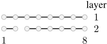
Proof. Let P = ([8],E1,E2) with E1 = {{i, i + 1} | i ∈ [7]} and E2 = E1 \ {{2, 3}} (see Figure 2). For the sake of contradiction, assume that (p1, p2) is a Nash equilibrium in Diff(P, 2). We distinguish two cases:
1) p1 ∈ [3] or p2 ∈ [3]: Let p1 = i ∈ [3]. Then, p2 = i+1, as this is the unique best response of player 2. Player 1 can improve by deviating to vertex i + 2.
2) p1 ∈ [4, 8] and p2 ∈ [4, 8]: If p1 = i ∈ [4, 5], then p2 = i + 1 is the unique best response of player 2 from the relevant interval [4, 8]. Player 1 can improve by choosing vertex 3. If p1 = 6, then p2 = 3 is the unique best response of player 2. If p1 = i ∈ [7, 8], then p2 = i-1 is the unique best response of player 2 from the relevant interval [4, 8]. Player 1 can improve by choosing vertex 3.
Intuitively, the reason why a disappearing edge is enough to prevent the existence of a Nash equilibrium on a temporal path is that players may want to play in the immediate surrounding of such a disappearing edge, in order to color some part of the temporal path that otherwise remains uncolored (in Figure 2, these are the vertices {1, 2}). However, if the disappearing edge is not located around the center, then the player close to this edge is at risk of loosing many vertices to the other player. This is in contrast to monotonically growing temporal graphs where edges are not allowed to disappear.
As a consequence of Theorem 4, it follows that Nash equilibria cannot be guaranteed for non-superset temporal paths when edges are allowed to disappear.
3.2 Temporal Cycles
In this section, we prove that in contrast to paths, a Nash equilibrium may fail to exist on a superset temporal cycle. However, enforcing that edges do not disappear over time is enough to guarantee the existence of a Nash equilibrium.
Superset Cycles
The guaranteed existence of a Nash equilibrium on superset temporal paths (Theorem 2) does not extend to superset temporal cycles despite the fact that as on superset paths all vertices will be colored in the end. This can be shown using the graph depicted in Figure 1 with an additional layer connecting all vertices to a cycle and a similar argument as in Theorem 1.
Theorem 5 (⋆). There is a superset temporal cycle C such that there is no Nash equilibrium in Diff(C, 2).
Monotonically Growing Cycles
If we require that edges do not disappear over time, then a Nash equilibrium is again guaranteed to exist:
Theorem 6 (⋆). On every monotonically growing temporal cycle C = ([n], (Ei)i∈[τ]) a Nash equilibrium in Diff(C, 2) can be found in O(τ · n) time.
As the proof of Theorem 6 is quite involved, we present only a high-level overview here. We start our description by making some definitions that are only relevant for temporal diffusion games:
Definitions. Let P = ([n], (Ei)i∈[τ]) be a temporal path and v1, v2 ∈ [n] with v1 ≤ v2. Let ℓ := v2 - v1 + 1. If ℓ is odd, then we call m := v1+⌊ ℓ2 ⌋ the central vertex of [v1, v2]. If ℓ is even, then we call ml := v1 + ℓ2 -1 and mr := v1 + ℓ2 central vertices of [v1, v2].
Without loss of generality, we assume that for a given temporal cycle C = ([n], (Ei)i∈[τ]), it holds that τ > 1 and that the last two layers differ, i.e., Eτ ̸= Eτ-1. For a temporal cycle C = ([n], (Ei)i∈[τ ]), we denote by F(C) the monotonically growing temporal linear forest that results from deleting the last layer from C, i.e., F(C) = ([n], (Ei)i∈[τ-1]).
In the proof of Theorem 6 (see full version), we look at two variants of temporal diffusion games, which are both zerosum games:
Temporal difference diffusion games (dDiff) A variant of temporal diffusion games where the payoff of a player is the difference between the number of vertices colored by her and the number of vertices colored by the other player.
Temporal lifetime difference diffusion games (ldDiff) A
variant of temporal difference diffusion games where only one diffusion step is carried out on the last layer.
The proof of Theorem 6 is split into two parts. In the first part, we prove the following lemma:
Lemma 1. Let C be a monotonically growing temporal cycle. A Nash equilibrium in dDiff(C, 2) is guaranteed to exist.
To prove the lemma, it is sufficient to find a Nash equilibrium in ldDiff(F(C), 2), as both players color the same number of vertices after step τ - 1 in dDiff(C, 2). We show that in all temporal lifetime difference diffusion games on monotonically growing temporal linear forests there always exists some non-empty set of vertices such that in case a player selects one of them, she always colors at least as many vertices as the other player. These are the nice central vertices:
Definition 1. Let F = ([n], (Ei)i∈[τ]) be a monotonically growing temporal linear forest. Let R be the maximum number of vertices that are reachable from any vertex in F until step τ . A vertex v is a nice central vertex if v reaches R vertices until step τ and if v is a central vertex of the set of vertices reachable from v until step τ .
Notably, each strategy profile where the players play on different nice central vertices is a Nash equilibrium in ldDiff(F, 2). In addition, we prove that if only one nice central vertex v exists, then (v, v + 1) is a Nash equilibrium.
In the second part of the proof, we show that at least one Nash equilibrium in dDiff(C, 2) described above is also a Nash equilibrium in Diff(C, 2).
Monotonically Shrinking Cycles
The example in Figure 2 can be modified to show that enforcing edges to only disappear over time is not enough to guarantee the existence of a Nash equilibrium on a temporal cycle (as in the case of temporal paths).
Theorem 7 (⋆). There is a monotonically shrinking temporal cycle C with two layers such that there is no Nash equilibrium in Diff(C, 2).
4 Temporal Voronoi Games
In this section, we study temporal Voronoi games. In contrast to temporal diffusion games, here, the color of a vertex v is determined solely by the temporal distances from the players' positions to v.
4.1 Monotonically Shrinking Paths and Cycles
In Section 2, we observed that temporal diffusion games and temporal Voronoi games might already differ on a simple temporal path. In contrast to this, both games are equivalent on monotonically shrinking temporal linear forests and cycles, as no foremost walk ever needs to wait at any vertex in these graphs.
Lemma 2. Let G = ([n], (Ei)i∈[τ]) be a monotonically shrinking temporal linear forest or cycle and let p1, p2 ∈ [n]. For strategy profile (p1, p2), the final coloring of the vertices is the same in Diff(G, 2) and in Vor(G, 2).
Proof. As already noted in Section 2, a vertex v colored with color i ∈ [2] in Vor(G, 2) is colored the same in Diff(G, 2), as pi reaching v first implies that pi also reaches every vertex on a foremost walk from pi to v first.
To see that on monotonically shrinking temporal linear forest and cycles the converse also holds, assume that v gets colored with color 1 in Diff(G, 2). Note that there is exactly one temporal walk from p1 to v which does not use vertex p2 and no vertex repeatedly. Since no foremost walk ever needs to wait in G and v is colored in color 1, this temporal walk must have fewer edges than any temporal walk from p2 to v. For the same reason, the walk from p1 to v consists of exactly td(p1, v) edges. Thus, td(p1, v) < td(p2, v).
In particular, using Lemma 2, we can transfer Theorem 4 and Theorem 7 to temporal Voronoi games:
Corollary 1. There is a monotonically shrinking temporal path P and a monotonically shrinking temporal cycle C both consisting of two layers such that there is no Nash equilibrium in Vor(P, 2) and no Nash equilibrium in Vor(C, 2).
4.2 Superset Paths and Cycles
In contrast to temporal diffusion games, a Nash equilibrium in a temporal Voronoi game on a superset temporal path may fail to exist. In fact, the underlying dynamics of temporal Voronoi games on superset temporal paths might be quite intriguing and far more complex than for temporal diffusion games (as highlighted in the next subsection).
Theorem 8. There is a superset temporal path P and a superset temporal cycle C such that there is no Nash equilibrium in Vor(P, 2) and no Nash equilibrium in Vor(C, 2).
Proof. Let P = ([8], (E1,E2)) be the temporal path from Figure 2. By Lemma 2 and the proof of Theorem 4, there is no Nash equilibrium in Vor(P, 2). By appending to P the last layer P2 five times, we can ensure that either every vertex is colored by some player until step seven or both players reach the same set of vertices until step seven. Appending any additional layers to P does not enable any player to color further vertices (however, some additional vertices may be colored gray). In particular, we may append a layer which is a complete path or cycle.
4.3 Monotonically Growing Paths
Our main result for temporal Voronoi games is the guaranteed existence of a Nash equilibrium on monotonically growing temporal paths. It is open whether this can be extended to all monotonically growing temporal cycles.
Theorem 9 (⋆). On every monotonically growing temporal path P a Nash equilibrium in Vor(P, 2) can be found in O(n2 ) time.
While the complete proof of Theorem 9 can be found in the full version, we give an overview of some key ingredients here. Subsequently, we always assume that the graph is a monotonically growing path P = ([n], (Ei)i∈[τ ]).
A vertex b ≤ v is called a left boundary of v if ⃗ τb > td(v, b), where ⃗ τb denotes the index of the first layer in which the edge {b-1, b} appears (or ∞ if b = 1). Symmetrically, a vertex b ≥ v is a right boundary of v if ⃗τb > td(v, b) with ⃗τb referring to the first appearance of {b, b + 1}. Note that 1, v, and n are always boundaries of v. The importance of boundaries arises from the following lemma.
Lemma 3. For three vertices v < w < x ∈ [n], td(v, x) = td(w, x) if and only if there exists a right boundary r of v with w ≤ r < x.
Proof. If there is such a right boundary r, then v will reach r + 1 at time ⃗τr. Clearly, the same holds for w. Therefore, td(v, x) = td(w, x) for all x > r.
Conversely, assume that td(v, x) = td(w, x) and let x be minimal with this respect. Since td(w, x - 1) < td(v, x - 1) ≤ td(v, x) - 1 = td(w, x) - 1 (i.e., w needed to wait at x - 1), we must have that ⃗τx-1 = td(w, x) = td(v, x) > td(v, x - 1), i.e., x - 1 is a right boundary of v.
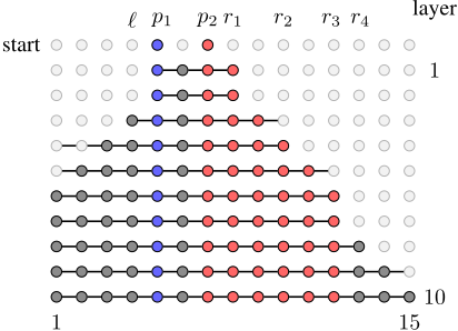
Let ℓ < ℓ′ be two left boundaries of a vertex v such that there is no other left boundary of v in between them. We call the interval [ℓ, ℓ′ [ ⊂ [n] a left boundary interval of v. The definition of right boundary intervals is analogous. Note that the boundary intervals of v partition [n]\{v}. For any w ̸= v, we write v(w) to denote the boundary interval of v which contains w. From Lemma 3, the following can be derived. For an example, consider Figure 3.
Lemma 4. Let P be a monotonically growing temporal path and p1, p2 ∈ [n]. In Vor(P, 2), it holds U1(p1, p2) ⊆ p2 (p1) and U2(p1, p2) ⊆ p1 (p2).
Proof. As all other cases are symmetric, we only show U1(p1, p2) ⊆ p2 (p1) and assume that p2 (p1) = ]r, r′ ] is a right boundary interval of p2. Thus, we have p2 ≤ r < p1 ≤ r′ . Lemma 3 implies that all vertices strictly to the right of r′ are colored gray. Further, as r is a right boundary of p2, p2 reaches r before the edge {r, r + 1} appears and thus before td(p1, r). This implies that neither r nor any vertex to the left of it is colored with color 1.
This allows us to easily find best responses:
Lemma 5. Let p1 be an arbitrary vertex and J be a largest boundary interval of p1. Then the vertex p2 ∈ J which is closest to p1 is a best response to p1.
Proof. For strategy profile (p1, p2), by Lemma 3, player 2 colors all vertices in J. By Lemma 4, the claim follows.
Starting with an arbitrary vertex v1 and iteratively applying Lemma 5, we obtain a sequence of vertices v1, v2, . . . , each being a best response to its predecessor. The following lemma then implies Theorem 9.
Lemma 6 (⋆). Let v1, v2, . . . be a best response sequence as defined above. Then there exists an index i ≤ n such that (vi, vi+1) is a Nash equilibrium.
5 Conclusion
Our work is meant to initiate further systematic studies of (not only competitive) games on (classes of) temporal graphs. There is a wealth of unexplored research directions to pursue.
An immediate and very concrete challenge from our work is to analyze whether a Nash equilibrium is guaranteed to exist in all temporal Voronoi games on monotonically growing temporal cycles. There are also many more special temporal graphs to study. Another direction is to consider variations of temporal diffusion and Voronoi games. For example, one could limit the time horizon such that players can only color vertices which they reach until the last layer (note that Theorem 2 does not hold in this case). Also, the payoff could be defined as the difference of the number of vertices colored by the players. It is also natural to study the games with more than two players or more initially chosen vertices. In addition, considering model variations already studied on static games such as "splitting" gray vertices between players is possible. Finally, for Voronoi games, there are several different temporal distance notions to consider. For example, one may study non-strict walks, for which Theorem 9 trivially holds (in fact, we have no example of a temporal graph without a Nash equilibrium in a non-strict Voronoi game).
Acknowledgements
Niclas Boehmer was supported by DFG project MaMu (NI 369/19). Malte Renken was supported by DFG project MATE (NI 369/17).
@inproceedings{ijcai2021p7,
  title     = {Two Influence Maximization Games on Graphs Made Temporal},
  author    = {Boehmer, Niclas and Froese, Vincent and Henkel, Julia and Lasars, Yvonne and Niedermeier, Rolf and Renken, Malte},
  booktitle = {Proceedings of the Thirtieth International Joint Conference on
               Artificial Intelligence, {IJCAI-21}},
  publisher = {International Joint Conferences on Artificial Intelligence Organization},
  editor    = {Zhi-Hua Zhou},
  pages     = {45--51},
  year      = {2021},
  month     = {8},
  note      = {Main Track},
  doi       = {10.24963/ijcai.2021/7},
  url       = {https://doi.org/10.24963/ijcai.2021/7},
}
TY - CPAPER TI - Two Influence Maximization Games on Graphs Made Temporal AU - Boehmer, Niclas AU - Froese, Vincent AU - Henkel, Julia AU - Lasars, Yvonne AU - Niedermeier, Rolf AU - Renken, Malte T2 - Proceedings of the Thirtieth International Joint Conference on Artificial Intelligence, IJCAI-21 PB - International Joint Conferences on Artificial Intelligence Organization PY - 2021 SP - 45 EP - 51 DO - 10.24963/ijcai.2021/7 UR - https://doi.org/10.24963/ijcai.2021/7 ER -Copied
Machine-readable versions of this paper, for tools and AI agents:





