Handling Overlaps When Lifting Gaussian Bayesian Networks

1 Introduction and RelatedWork

Modeling real-world systems in areas such as healthcare, biostatistics, or financial markets requires formalisms to use continuous variables and relationships among them. These areas may also involve many objects in relation to each other, affected by uncertainties. Probabilistic graphical models (PGMs) such as Bayesian Networks (BNs) have been used to model conditional independence assumptions regarding these random variables (randvars) [Koller et al., 2009]. Being able to efficiently answer queries in these models, also often referred to as inference, has triggered a lot of research [Zhang and Poole, 1996; Blei et al., 2017; Salmer´on et al., 2018].

To handle many objects efficiently, Poole [2003] introduces first-order probabilistic inference, which exploits symmetries in a model by combining indistinguishable instances using logical variables (logvars) to reason with representatives for the represented instances. Using a compact representation and performing inference with representatives is also referred to as lifting and has been an active research field in the past years [Kimmig et al., 2015; Sharma et al., 2018; Holtzen et al., 2019]. For a discrete PGM, Taghipur et al.

[2013] present a lifted variable elimination algorithm and Braun and M¨oller [2016] a lifted version of the junction tree algorithm by Lauritzen and Spiegelhalter [1988]. In the continuous setting, Choi et al. [2010] present a lifted version for variable elimination in factor graphs with Gaussian pairwise potentials. Hartwig and M¨oller [2020] apply the concept of lifting to Gaussian Bayesian networks (GBNs), which have been introduced by Shachter and Kenley [1989] and widely applied across multiple fields [Cano et al., 2004; Grzegorczyk, 2010; Huang et al., 2011; Froelich, 2015].

The current approach by Hartwig and M¨oller [2020] forbids overlaps between logvar sequences, which reduces the applicability dramatically. This paper extends the approach by generalizing existing and developing new algebraic operations to handle overlaps. Example 1 contains a simple scenario that currently cannot be handled in a lifted way, but will be supported by the techniques introduced in this paper.

Example 1 (Simple GBN with overlaps). Patients (P) have a disease severity level (S) which is influenced by getting a specific dose (D) of a medicine (M). Each medicine (M) has an effectiveness (E). The logvars here are the patients (P) and the medicines (M). The logvars combined with the randvars group together isomorphic instances of patients getting doses of medicine and medicines being effective, leading to so called parameterized randvars (PRVs) E(M), D(P, M), and S(P). Overlaps are present if PRVs share the same logvar, e.g., D(P,M) and E(M) share logvar M. The GBN puts the PRVs into relation in the form of E(M) → D(P,M) → S(P ), where M as well as P overlap between PRVs.

Specifically, this paper contributes (i) a lifted representation of the joint distribution of a Gaussian BN with symmetries, allowing overlaps in logical variables and (ii) a lifted query answering approach using this lifted joint. Complexity analyses and experimental results show that - despite overlaps - constructing and answering queries on the lifted joint outperform their grounded counterparts significantly.

The remainder of the paper is structured as follows. Section 2 describes preliminary definitions and recaps the lifting approach by Hartwig and M¨oller [2020]. Section 3 presents the construction of the lifted joint, Section 4 introduces the updated rules for arithmetic operations with the lifted joint, and Section 5 explains query answering. Section 6 and Section 7 present a theoretical and experimental look at the contributions. We end with the conclusion and next steps.

2 Preliminaries and Notations

This section covers notations and summarizes the result of the work by Hartwig and M¨oller [2020]. Notation-wise, we follow Taghipour et al. [2013], Braun and M¨oller [2016], and Hartwig and M¨oller [2020]. Throughout this paper, we use bold symbols for vectors, sets, sequences, and matrices, and thin symbols for scalars or individual elements. In abuse of notation, we use set operations for sequences, where we apply the operation to the set containing the sequence elements.

2.1 Gaussian Bayesian Networks

Based on BNs this section defines GBNs and specifies their semantics.

Definition 1. ABN is a directed acyclic graphwhose vertices represent N randvars Vt ∈ V with t = 1, ...,N and whose edges U ⊂ (V,V) represent the dependencies between the randvars. The set of parents Pa(Vt) of a randvar Vt ∈ V is defined as the set of randvars that have a directed edge to Vt.

Definition 2. A GBN is a BN where all randvars are continuous and normally distributed. The edges represent linear relationships between the randvars. As in BNs, the joint density can be factorized using the conditional probability densities of Vt, t = 1, ..., N given it parents Pa(Vt):

where µVk and µVt are marginal means, σ2Vt is the node variance, and βVk,Vt represents the influence of parent Vk on its child Vt.

The joint probability distribution P(V) over randvars V is defined by a multivariate Gaussian distribution: P(V) = N (µ,Σ), where µ denotes the mean vector and Σ the covariance matrix. This distribution can be constructed from a GBN using the algorithm by Shachter and Kenley [1989], which requires a topological ordering of the randvars in the GBN. They use a transition matrix, here denoted as T , where a non-zero entry at Tk,t = βk,t means that there is a parentchild relationship between Vk and Vt. The matrix T simply contains all β values to allow for matrix operations. The covariance matrix Σ is inductively built using T . It is for any t and s = 1, ..., t - 1:Σ11 = σV1 (2)

2.2 ParameterizedModels

The idea of parameterized models is to work with representatives for a group of randvars sharing a probability distribution and parents. Logvars identify groups and parameterize randvars to represent a set of isomorphic randvars. The aim of lifting is to work solely with PRVs as representatives for the randvars belonging to the PRV.

Definition 3. Let V be a set of randvars and L be a set of logvar names. A PRV X is a syntactical construct of a randvar V ∈ V combined with a sequence of logvars L ⊆ L into V (L) to represent a set of randvars. If L = ∅, the PRV is parameterless and constitutes a propositional randvar. The domain D(L) = {l1 , ..., lH } contains the instances of logvar L. The domain of a sequence of logvars is defined as D(L) = ×L∈LD(L). Grounding a PRV X with a logvar L results in a set of randvars gr(X) = {Vl1 , ..., VlH}.

Each PRV X also has a range denoted as range(X) that contains the possible values of X. Since we work with continuous normally distributed randvars, range(X) = R in general. Instead of a discrete conditional probability table, we specify a mean η and variance λ for each PRV X.

2.3 Parameterized Gaussian Bayesian Networks

Instead of N ground randvars V, a parameterized GBN contains M PRVs X. Each PRV Xi ∈ X, i = 1, ...,M, has a PRV mean ηi and a variance λi. Each edge between a parent Xu and a child Xs has a linear influence βXu,Xs that describes the linear relationship between the PRVs analogously to the propositional GBN of Definition 2. Grounding a PRV Xi leads to a set of ground randvars Vi = gr(Xi) with |Vi| = |D(Li)| that have the same mean and variance. Grounding a topologically ordered list of PRVs results in a topologically ordered list of ground randvars because the parent-child relationships for each ground randvar are defined by the parent-child relationships of the corresponding PRV. A propositional randvar V can be interpreted as a PRV V (L) with |D(L)| = 1. There are three different kinds of relationships between two PRVs Xi and Xj :

No parent: A PRV has no parent PRV, resulting in no influencing factors on the PRV.

Disjoint logvar sets: The logvars Li of the parent PRV Xi and the logvars Lj of the child PRV Xj are disjoint. Disjoint logvar sets result in a relationship from every randvar in gr(Xi) to every randvar in gr(Xj).

Overlapping logvar sets: The logvars Li of the parent PRV Xi and the logvars Lj of the child PRVXj overlap, i.e., Lshared := Li ∩Lj ̸= ∅. Grounding results in a relation where each child node is influenced by all |D(Li \ Lj)| parents that share the same grounding of Lshared.

For ease of notation, we assume a global sorting Ω of all model logvars such that every logvar sequence uses the global sorting for ordering its logvars. This sorting places no restriction on the expressivity of the model. In the course of this paper, we need the following three helper functions.

Definition 4. For two sequences of logvars Li and Lj, we define a function seq(Li,Lj) that returns the combined sequence of logvars according to the global sorting Ω. Given L ∈ seq(Li, Lj), we define

2.4 Queries

Query answering concerns queries for (conditional) marginal probabilities or distributions of a set of randvars (given a set of events as evidence), defined as follows.

Definition 5. A query P(Q|E = e) consists of a query set Q ⊆ V and a set of events {Eh = eh}Oh=1 with eh ∈ R where Eh ∈ V and O is the number of observations.

2.5 Current Lifting Approach

Hartwig and M¨oller [2020] lift the algorithm by Shachter and Kenley [1989] for parameterized GBNs with disjoint logvar sets between parent and child nodes. The lifted representation of the covariance matrix is given by the M-dimensional vector λ and the M ×M-dimensional matrix ρ, where λ is filled with the individual λ values of the PRVs and all elements of ρ are calculated as follows without groundings:

where δ is the Kronecker delta function that equals one if Xu = Xj . The lifted representation can be grounded by

where lif(Vs) refers to the PRV that contains the specific ground randvar Vs.

Equation (8) makes it apparent that overlaps are excluded as it posits that all groundings of a parent PRV have connections to all groundings of the child PRV. This all-to-all connection does not happen when overlaps occur in the two logvar sequences. With this limitation, answering a query P(Q|E = e) is done using lifted operations for matrix multiplication and inversion together with

For details on how to come up with the closed form for conditional Gaussian distributions, see, e.g., Eaton [1983].

3 Handling Overlaps in the Lifted Joint

When allowing overlaps between the logvars of a parent and a child PRV, connections from parent to child grounding only exist if the groundings share the same instances of the overlapping logvars. This violates the assumptions about disjoint logvars, causing that Eq. (8) no longer holds. Therefore, we need to specify the general form of the transition matrix T given overlaps and construct a lifted representation of the covariance matrix anew.

The main result of this section is a lifted representation for the values in the covariance matrix in the form of M ·M lifted covariance vectors, where each covariance vector ρ(i,j) has a dimensionality of 2Li∩Lj , which does not depend on the domain sizes, together with a lifted construction approach to get the lifted representation. Specifically, this section derives the main result and shows that the lifted representation is an exact alternative representation that exploits the structure imposed by isomorphic randvars. For brevity: If we index the covariance matrix Σ with a PRV index, we refer to the block in the covariance matrix belonging to the PRV.

3.1 General Form of the TransitionMatrix

The transition matrix T can be structured into M × M blocks. Each block Ti,j describes the relationships between all randvars represented by Xi and all randvars represented by Xj. As the randvars are isomorphic, we can proceed block-wise instead of line-wise in Eqs. (2) to (5). In the non-overlapping case, a block contains either zeroes, namely, if there is no parent-child relationship between Xi and Xj, or the same entries denoted as βi,j resulting in an equation T i,j = βi,jJ|D(Li)|×|D(Lj)| for a block, where J denotes the all-ones matrix. For a full overlap, each randvar in gr(Xi) has a connection to only one randvar in gr(Xj), namely, where Xi and Xj are grounded with the same instances. Given a global ordering, a full overlap results in a block design of Ti,j = βi,jI|D(Li)|×|D(Lj)|. Given a full overlap, we could add non-overlapping logvars. Adding a non-overlapping additional logvar Lp in the parent sequence implies that previously one randvar is now replaced by |D(Lp)| randvars, which leads to a Kronecker multiplication of a J|D(Lp)|×1 column vector (parent variables correspond to rows). Analogously, a non-overlapping additional logvar Lc in the child PRV results in a Kronecker multiplication of a J1×|D(Lc)| row vector. Depending on the global ordering of the logvars, we get the following general formula for T , with J0 = I:

3.2 Constructing the Covariance Matrix

The lifted representation of the transition matrix T allows for calculating a lifted version of the covariance matrix Σ as the dimensions of the blocks are determined by the logvars in the same way. The critical steps are Eqs. (3) and (5), which are inductive formulations. Therefore, we use an inductionlike approach to show that all blocks follow a fixed structure, which enables a lifted Σ.

During construction and query answering, we will need to iterate over all possible combinations of J and I for a logvar sequence L. For ease of notation, we use that J1 = J and J0 = I and iterate over a binary vector q from 0 = 0 . . . 0 (all I) to 1 = 1 . . . 1 (all J) for L to use as exponents to J as basis. The term Q refers to the set of all possible permutations. Each position in q can be mapped to the corresponding logvars in L. A superscript i means that q(i) refers to logvars Li, a superscript (i, j) refers to the logvars in Li ∩ Lj. Without an overlap, we set q to 1. In slight abuse of notation, we use a projection πL(q) to mean projecting q onto those entries that are mapped to logvars in L. Similarly, a selection σq(Q′ ) yields those vectors q′ in Q′ where q′ , projected onto the shared logvars with q, has the same values as q.

The assumed structure of an on-diagonal block in Σ, representing the relationship of PRVXi with itself, is

for which we have to store the 2|Li| -dimensional vector ρ(i) .

For Xi, Xj , we assume the following off-diagonal structure:

with

Equation (13) is a special case of Eq. (14) as both logvar sequences involved are equal, i.e., q(i,j) = q(i) , seq(Li, Li) = Li, and dim and qexp simplifying to their first cases.

Next, we show that, given the assumed structures, all blocks added to the covariance matrix follow the same format. The formula for a new block is.

Inserting Eqs. (12) and (14) into Eq. (16) for one arbitrary summand n = k results in

For the combinations of Li, Lk, and Lj, there are seven possible cases (for brevity, we write ℓ = |D(L)|):

1. L ∈ Lj ∩Lk and L /∈ Li, result: IℓJℓ×1 = Jℓ×1
2. L ∈ Lj and L /∈ Lk ∪Li, result: Jℓ×1 · 1 = Jℓ×1
3. L ∈ Lk ∩Li and L /∈ Lj, result: J1×ℓIℓ = J1×ℓ
4. L ∈ Li and L /∈ Lk ∪Lj, result: 1 · J1×ℓ = J1×ℓ
5. L ∈ Lk and L /∈ Li ∪Lj, result: J1×ℓJℓ×1 = ℓ
6. L ∈ Lj ∩Lk ∩Li, result: IℓIℓ = Iℓ
7. L ∈ Li ∩Lj and L /∈ Lk, result: Jℓ×1J1×ℓ = Jℓ×ℓ

Cases 1 and 2 result in the same kron factor, independently of Lk. The same holds for Cases 3 and 4. Case 5 requires a |D(L)| factor for all summands, which does not affect the structure. Cases 6 and 7 depend on Lk. Both cases are taken care of in Eq. (14) as whenever Li ∩ Lj ̸= ∅, we keep the corresponding logvars in the summation index. Every entry of the new ρ(i,j) vector can be calculated as follows.

The transpose calculation in Eq. (4) stays in the same structure given by Eq. (14):

Based on the formula for calculating a new off-diagonal block, we apply Eq. (5) to calculate a new on-diagonal block. The only difference to the off-diagonal case is that we additionally add the PRV variance λXj to the diagonal after calculating the ρ vector using Eq. (18), meaning, we add PRV variance λXj to the one summand indexed by 0 . . . 0:

The last part of our induction-like proof is to show that our starting point is in line with our assumptions. Based on the definition by Shachter and Kenley [1989], we know that Σ11 = λX1 I, which is a specific case of the general form from Eq. (2), where only ρ(1) 0...0 has a value unequal to zero.

3.3 Lifted Representation

With Λ as the overall number of logvars, we can record that the lifted representation requires

1. M · M lifted covariance vectors, where each covariance vector ρ(i,j) has a dimensionality of 2|Li∩Lj| ,
2. anM-dimensional mean vector η,
3. a Λ-dimensional cardinality vector τ for the logvars, and
4. aM×Λ-dimensional mapping ψ fromPRVs to involved logvars.

Based on Eq. (14), we can convert the lifted representation of the covariance matrix back into a grounded representation. Given the lifted joint of the full joint distribution represented by a parameterized GBN and a fully lifted construction, we now have to specify arithmetic operations for working with the lifted joint, which we need for lifted query answering.

4 Arithmetic Operations in the Lifted Joint

Since handling overlaps results in a more complex lifted representation of the joint distribution, we need new rules for working with this lifted representation to support lifted query answering. Adding or subtracting two blocks with matching dimensions as well as a summation over the same index set is straight-forward, i.e., the corresponding ρ values are added or subtracted. Multiplication and inversion are more complex and we show next how to handle them.

4.1 Multiplication

Multiplying two blocks Σi,j,Σj,k of the same structure of Eq. (14) boils down to a repeated application of Eq. (17) because every summand of Σi,j is multiplied with every summand of Σj,k, and every individual summand of Σj,k has the same structure as the T matrix, meaning we can calculate the ρ-value of the resulting matrix in a lifted way as follows:

with or(q(i,j) , q(j,k) ) as the bitwise or-operation, a function id that returns 1 if the resulting logvar sequence of the oroperation is identical to the values in q(i,k) at the logvar positions referenced in q(i,k) , i.e.,

and a function lexp

which returns 1 if the referenced logvar L fulfils both parts of a conjunction. The first part asks that L occurs only in Lj and not Li or that the value of L in q(i,j) is 1, which can only happen if the first disjunct is false. The second part asks the same regarding k instead of i. The returned value as an exponent ensures that the factor of the domain size |D(L)| occurs whenever two J's meet.

The main idea of Eq. (21) is to take into account all possible combinations of J and I matrices that occur in the summations of both blocks. Block matrix equation rules allow us to use Eq. (21) also for multiplying rows or matrices of structured blocks as long as the dimensions are matching.

4.2 Inversion

In the non-overlapping case, Hartwig and M¨oller [2020] use the recursive block matrix inversion approach by Bernstein [2009], that we transfer to this case where overlaps are allowed:

where

This approach needs to be able to perform matrix multiplication, which we have already described and a way to invert blocks in the structure of on-diagonal blocks (see Eq. (13)). For this inversion, we use the lemma by Searle and Henderson [1979], for which they provide a detailed deduction and proof in their work:

Lemma 1. Given

of order Np = ∏pr=1 nr where qi refers to the entries in q and ni to each dimension, the inverse is given by

where

and

With Lemma 1, lifted subtraction, and lifted matrix multiplication, we can now perform a block matrix inversion to invert the full covariance matrix in a lifted way.

5 Lifted Query Answering

A query P(Q|E = e) as given in Definition 5 involves a query set Q and evidence E = e. Equations (10) and (11) describe the formulas for determining the posterior distribution N(µ∗ ,Σ∗ ). The involved matrices ΣQE, ΣEE, and ΣEQ are sub-matrices of the overarching Σ matrix. Not all sub-matrices follow the structure of Eq. (14). The structure occurs if all ground observations E and query randvars Q refer to the same set of logvar instances for all shared logvars. We call the query to be liftable if E and Q fulfill this condition. Then, ρlif(E) contains only a subset of ρ vectors and the cardinality for all operations is reduced to the logvar cardinality occurring in the query. Using the lifted representation combined with the lifted operations for multiplication and inversion described in Section 4, a lifted representation ρ∗ for the matrix Σ∗ can be generated. To get the grounded query answer Σ∗ , ρ∗ can simply be grounded. The µ∗ needs to be calculated grounded because it involves grounded evidence. We can ground ΣQEΣ-1 EE and multiply it with the vector e - µE to get µ∗ .

6 Complexity

We discuss the runtime complexity of constructing the lifted joint and using it for query answering. As stated above we have N randvars, combined into M PRVs, using Λ logvars. We use S to denote the longest occurring logvar sequence.

6.1 Constructing the Lifted Joint

For constructing the ground level covariance matrix in the joint distribution, we have an upper bound of O(N 3 ). Our lifted approach is fully independent of N, because we directly iterate over M PRVs. Allowing for overlaps results in iterations over binary vectors. We need to potentially iterate over O(2Λ) permutations, resulting in an overall runtime complexity of O(M 3 2Λ). Since M ≪ N and 2Λ ≪ N with decent domain sizes, it is a significant improvement.

6.2 Lifted Query Answering

We denote the number of queried randvars as NQ and the number of evidence randvars as NE. Furthermore, we refer to the number of PRVs involved in the NQ and NE randvars usingMQ andME, respectively.

Matrix multiplication and inversion drive the complexity of query answering. Although there are matrix inversion and multiplication algorithms that have a runtime complexity of less than O(N 3 ), for the sake of simplicity, we take O(N 3 ) as an upper bound [Le Gall, 2014], which results in a runtime complexity of O(N 3E +N 2E NQ+NEN 2Q). Depending on the set sizes, one of the terms dominates the other.

In the lifted case, multiplying two blocks of size 2S has a complexity of O(22S ) because in the worst case we need to iterate fully through all possible I, J combinations. Thus, the matrix multiplications operations have complexity of O(M 2EMQ22S ) and O(MEM 2Q22S ). The inversion of one individual block on the diagonal of the covariance matrix involves the multiplication of two matrices, both with at most 2S × 2S dimensions, resulting in a complexity of O(23S ). In the block matrix inversion, we have at most ME recursive function calls and Kronecker component block multiplications of at most ME blocks, resulting in a combined inversion complexity of O(ME23S + M 2E 2S ).

To calculate the mean vector, we still have ground operations. However, the dependency on both NQ and NE is only linear: Grounding the result of ΣQEΣ-1 EE is in O(NQNE) and multiplying the result with the ground level evidence vector e - µE is in O(NQNE), as well.

Overall, this results in a complexity of O(M 2EMQ22S + MEM 2Q22S + ME23S + NQNE). Unfortunately, the last term means that query answering is not fully lifted. Compared to the non-overlapping case, NQ now also appears as a ground term. We cannot really avoid NE because to incorporate ground evidence, we always need to at least visit each evidence randvar once. The dependency on NQ might be a focus for further research, though.

7 Experimental Evaluation

We demonstrate the complexity results by evaluating constructing the lifted joint and answering queries.

We set up an experiment with 4 PRVs and 5 logvars that are partially shared. We increase the domain sizes of 2 logvars in exponential steps (from 2 to 27 ) resulting in around 20,000 randvars in the grounded model for the largest domains. For conditional query answering, we introduce evidence for the majority of the randvars and use a query set of 4 randvars.

Figures 1 and 2 show the results. For both benchmarks, the lifted version is significantly faster. Similar to the results by Hartwig and M¨oller [2020], construction is independent of the domain sizes of the logvars (i.e., the number of grounded randvars) and query answering shows some dependence on the number of evidence randvars. The results also show that working with the more complex structure of representing blocks in the covariance matrix with ρ comes with additional overhead recognizable in the low cardinality cases.

In summary, the runtimes reflect that models with overlaps in the logvar sequences make constructing and query an- Cardinality of logvars in evidence PRVs swering more complex compared to models without overlaps. However, applicability of the approach increases immensely. Additionally, compared to the ground case, the lifted version gains dramatically in terms of runtime.

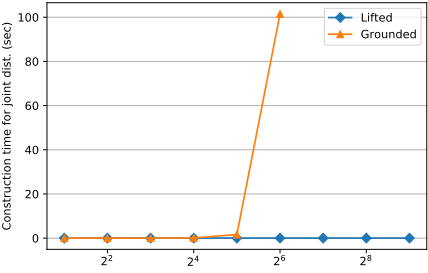
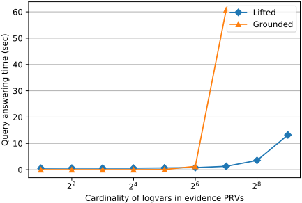
Figure 2: Runtimes for query answering

8 Conclusion and Outlook

We present a generalized approach to lifting GBNs, consisting of constructing a lifted joint and lifted query answering using the lifted joint. Whereas previous work lifts the inductive construction approach of the full joint of a GBN only for parameterized GBNs that do not have overlaps in the logvars, the presented approach works for parameterized GBNs where no restrictions are placed on the logvars, which goes beyond liftability results of discrete models, is however tied to the continuous setting. Allowing overlaps, we significantly extend the applicability of lifting in GBNs. We show that constructing a lifted joint and answering queries on the lifted joint leads to savings in terms of complexity. The experimental results show that this theoretical speed-up can also accomplished in an implementation with impressive results.

For future work, we look into lifting evidence handling as well as query answering with parameterized queries as done for discrete parameterized models [Taghipour et al., 2013; Braun and M¨oller, 2018] targeting the O(NENQ) term. Another avenue concerns hybrid models where continuous and discrete randvars simultaneously occur in the model.