On the Parameterized Complexity of Polytree Learning

1 Introduction

Bayesian networks are the most important tool for modelling statistical dependencies in joint probability distributions. A Bayesian network consists of a DAG (N,A) over the variable set N and a set of condiditional probability tables. Given a Bayesian network and the observed values on some of its variables, one may infer the probability distributions of the remaining variables under the observations. One of the drawbacks of using Bayesian networks is that this inference task is NP-hard. Moreover, the task of constructing a Bayesian network with an optimal network structure is NP-hard as well, even on very restricted instances [Chickering, 1995]. In this problem, we are given a local parent score function fv : 2N\{v} → N0 for each variable v and the task is to learn a DAG (N, A) such that the sum of the parent scores over all variables is maximal.

∗Contact Author

†Supported by the Deutsche Forschungsgemeinschaft (DFG), project OPERAH, KO 3669/5-1.

In light of the hardness of handling general Bayesian networks, the learning and inference problems for Bayesian networks fulfilling some specific structural constraints have been studied extensively [Pearl, 1989; Korhonen and Parviainen, 2013; Korhonen and Parviainen, 2015; Gr¨uttemeier and Komusiewicz, 2020; Ramaswamy and Szeider, 2021].

One of the earliest special cases that has received attention are tree networks, also called branchings. A tree is a Bayesian network where every vertex has at most one parent. In other words, every connected component is a directed in-tree. Learning and inference can be performed in polynomial time on trees [Chow and Liu, 1968; Pearl, 1989]. Trees are, however, very limited in their modeling power since every variable may depend only on at most one other variable. To overcome this problem, a generalization of branchings called polytrees has been proposed. A polytree is a DAG whose underlying undirected graph is a forest. An advantage of polytrees is that the inference task can be performed in polynomial time on them [Pearl, 1989; Guo and Hsu, 2002]. POLYTREE LEARNING, the problem of learning an optimal polytree structure from parent scores, however, remains NP-hard [Dasgupta, 1999]. We study exact algorithms for POLYTREE LEARNING.

Related Work. POLYTREE LEARNING is NP-hard even if every parent set with strictly positive score has size at most 2 [Dasgupta, 1999]. Motivated by the contrast between the NP-hardness of POLYTREE LEARNING and the fact that learning a tree has a polynomial-time algorithm, the problem of optimally learning polytrees that are close to trees has been considered. More precisely, it has been shown that the best polytree among those that can be transformed into a tree by at most k edge deletions can be found in nO(k) |I|O(1) time [Gaspers et al., 2015; Safaei et al., 2013] where n is the number of variables and |I| is the overall input size. Thus, the running time of these algorithms is polynomial for every fixed k. As noted by Gaspers et al. [2015], a brute-force algorithm for POLYTREE LEARNING would need to consider nn-2 · 2n-1 directed trees. Polytrees have been used, for example, in image-segmentation for microscopy data [Fehri et al., 2019].

Our Results. We obtain an algorithm that solves POLYTREE LEARNING in 3n · |I|O(1) time. This running time is a substantial improvement over the brute-force algorithm mentioned above, thus positively answering a question of Gaspers et al. [2015] on the existence of such algorithms. We then study whether POLYTREE LEARNING is amenable to polynomial-time data reduction that shrinks the instance I if |I| is much bigger than n. We show that such a data reduction algorithm is unlikely. More precisely, we show that (under standard complexity-theoretic assumptions) there is no polynomial-time algorithm that replaces any n-variable instance I by an equivalent one of size nO(1) . In other words, it seems necessary to keep an exponential number of parent sets to compute the optimal polytree.

We then consider a parameter that is potentially much smaller than n and determine whether POLYTREE LEARNING can be solved efficiently when this parameter is small. The parameter d, which we call the number of dependent variables, is the number of variables v for which at least one entry of fv is strictly positive. The parameter essentially counts how many variables might receive a nonempty parent set in an optimal solution. We show that POLYTREE LEARNING can be solved in polynomial time when d is constant but that an algorithmwith running time g(d) · |I|O(1) is unlikely for any computable function g. Consequently, in order to obtain positive results for the parameter d, one needs to consider further restrictions on the structure of the input instance. We make a first step in this direction and consider the case where all parent sets with a strictly positive score have size at most p. Using this parameterization, we show that every input instance can be solved in 2ωdp · |I|O(1) time where ω is the matrix multiplication constant. With the current-best known value for ω this gives a running time of 5.18dp · |I|O(1) . We then consider again data reduction approaches. This time we obtain a positive result: Any instance of POLYTREE LEARNING where p is constant can be reduced in polynomial time to an equivalent one of size dO(1) . Informally, this means that if the instance has only few dependent variables, the parent sets with strictly positive score are small, and there are many nondependent variables, then we can identify some nondependent variables that are irrelevant for an optimal polytree representing the input data. We note that this result is tight in the following sense: Under standard complexity-theoretic assumptions it is impossible to replace each input instance in polynomial time by an equivalent one with (d + p)O(1) variables. Thus, the assumption that p is a constant is necessary.

2 Preliminaries

Notation. An undirected graph is a tuple (V,E), where V is a set of vertices and E ⊆ {{u, v} | u, v ∈ V } is a set of edges. Given a vertex v ∈ V , we define NG(v) := {u ∈ V | {u, v} ∈ E} as the neighborhood of v. A directed graph is a tuple (N, A), where N is a set of vertices and A ⊆ N×N is a set of arcs. If (u, v) ∈ A we call u a parent of v and v a child of u. Given a vertex v, we let P A v := {u | (u, v) ∈ A} denote the parent set of v. The skeleton of a directed graph (N,A) is the undirected graph (N, E) where {u, v} ∈ E if and only if (u, v) ∈ A or (v, u) ∈ A. A directed acyclic graph is a polytree if its skeleton is a forest, that is, the skeleton is acyclic [Dasgupta, 1999]. As a shorthand, we write P ×v := P × {v} for a vertex v and a set P ⊆ N.

Problem Definition. Given a vertex set N, a family F := {fv : 2N\{v} → N0 | v ∈ N} is a family of local scores for N. Intuitively, fv(P) is the score that a vertex v obtains if P is its parent set. Given a directed graph D := (N, A) we define score(A) := ∑v∈N fv(P A v ). We study the following computational problem.

POLYTREE LEARNING

Input: A set of vertices N, local scores F = {fv | v ∈ N}, and an integer t ∈ N0.

Question: Is there an arc-set A ⊆ N × N such that (N, A) is a polytree and score(A) ≥ t?

Given an instance I := (N,F, t) of POLYTREE LEARNING, an arc-set A is a solution of I if (N,A) is a polytree and score(A) ≥ t. Without loss of generality we may assume that fv(∅) = 0 for every v ∈ N [Gr¨uttemeier and Komusiewicz, 2020].

Solution Structure and Input Representation. We assume that the local scores F are given in non-zero representation. That is, fv(P) is part of the input if it is different from 0. For N = {v1, . . . , vn}, the local scores F are represented by a two-dimensional array [Q1,Q2, . . . ,Qn], where each Qi is an array containing all triples (fvi (P), |P|, P) where fvi (P) > 0. The size |F| is defined as the number of bits needed to store this two-dimensional array. Given an instance I := (N, F, t), we define |I| := n + |F| + log(t).

For a vertex v, we call PF(v) := {P ⊆ N \{v} | fv(P) > 0} ∪ {∅} the set of potential parents of v. Given a yesinstance I := (N,F, t) of POLYTREE LEARNING, there exists a solution A such that P A v ∈ PF(v) for every v ∈ N: If there is a vertex with P A v ̸∈ PF(v) we can simply replace its parent set by ∅. The running times presentend in this paper will also be measured in the maximum number of potential parent sets δF := maxv∈N |PF(v)| [Ordyniak and Szeider, 2013].

A tool for designing algorithms for POLYTREE LEARNING is the directed superstructure [Ordyniak and Szeider, 2013] which is the directed graph SF := (N,AF) with AF := {(u, v) | ∃P ∈ PF(v) : u ∈ P}. In other words, there is an arc (u, v) ∈ AF if and only if u is a potential parent of v.

Parameterized Complexity. A problem is in the class XP for a parameter k if it can be solved in |I|g(k) time for some computable function g. In other words, a problem is in XP if it can be solved within polynomial time for every fixed k. A problem is fixed-parameter tractable (FPT) for a parameter k if it can be solved in g(k) · |I|O(1) time for some computable g. If a problem is W[1]-hard for a parameter k, then it is assumed to not be fixed-parameter tractable for k. A problem kernel is an algorithm that, given an instance I with parameter k computes in polynomial time an equivalent instance I ′ with parameter k′ such that |I ′ | + k′ ≤ h(k) for some computable function h. If h is a polynomial, then the problem admits a polynomial kernel. Strong conditional running time bounds can also be obtained by assuming the Exponential Time Hypothesis (ETH), a standard conjecture in complexity theory [Impagliazzo et al., 2001]. For a detailed introduction into parameterized complexity we refer to the standard textbook [Cygan et al., 2015].

3 Parameterization by the Number of Vertices

In this section we study the complexity of POLYTREE LEARNING when parameterized by n, the number of vertices. Note that there are up to n·2n-1 entries in F and thus, the total input size of an instance of POLYTREE LEARNING might be exponential in n.

Theorem 1. POLYTREE LEARNING can be solved in 3n · |I|O(1) time.

Proof. Let I := (N,F, t) be an instance of POLYTREE LEARNING. We describe a dynamic programming algorithm to solve I. We suppose an arbitrary fixed total ordering on the vertices of N. For every P ⊆ N, and every i ∈ [1, |P|], we denote with pi the ith smallest element of P according to the total ordering.

The dynamic programming table T has entries of type T[v, P, S, i] with v ∈ N, P ∈ PF(v), S ⊆ N \ (P ∪ {v}), and i ∈ [0, |P|].

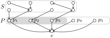
Each entry stores the maximal score of an arc set A of a polytree on {v} ∪ P ∪ S where v has no children, v learns exactly the parent set P under A, and for each j ∈ [i+1, |P |], only the arc (pj, v) is incident with pj under A. See Figure 1 for an illustration.

We initialize the table T by setting T[v, P, ∅, i] := fv(P) for all v ∈ N, P ∈ PF(v), and i ∈ [0, |P |]. The recurrence to compute an entry for v ∈ N, P ∈ PF (v), S ⊆ N \(P ∪{v}), and i ∈ [1, |P|] is

Note that the two vertex sets P ∪ (S \ S′ ) ∪ {v} and P ′ ∪ (S′ ∪ {pi}) \ (P ′ ∪ {v′ }) ∪ {v′ } = S′ ∪ {pi} share only the vertex pi. Hence, combining the polytree on these two vertex sets results in a polytree.

If i is equal to zero, then the recurrence is

Thus, to determine if I is a yes-instance of POLYTREE LEARNING, it remains to check if T[v, P,N \ (P ∪ {v}), |P|] ≥ t for some v ∈ N and some P ∈ PF(v). The corresponding polytree can be found via traceback. The correctness proof is straightforward and thus omitted.

The table T has 2n ·n2 ·δF entries. Each of these entries can be computed in 2|S| · n2 · δF . Consequently, all entries can be computed in ∑ni=0 (ni )2i · |I|O(1) = 3n · |I|O(1) time in total. To evaluate if there is some v ∈ N and some P ∈ PF(v) such that T[v, P,N \ (P ∪ {v}), |P|] ≥ t can afterwards be done in O(n · δF) time. Hence, the total running time is 3n · |I|O(1) .

The proof is closely related to a similar kernel lower bound for BAYESIAN NETWORK STRUCTURE LEARNING parameterized by n [Gr¨uttemeier and Komusiewicz, 2020].

Theorem 2. POLYTREE LEARNING does not admit a polynomial kernel when parameterized by n, unless NP ⊆ coNP/poly.

4 Dependent Vertices

We now introduce a new parameter d called number of dependent vertices. Given an instance (N,F, t) of POLYTREE LEARNING, a vertex v ∈ N is called dependent if there is a nonempty potential parent-set P ∈ PF(v). Thus, a vertex is dependent if it might learn a nonempty parent set in a solution. A vertex that is not dependent is called nondependent vertex. Observe that d is potentially smaller than n. We start with a simple XP-result.

Theorem 3. POLYTREE LEARNING can be solved in (δF)d · nO(1) time.

Proof. Choose for each dependent vertex vi one of its potential parent sets Pi ∈ PF(vi) and check afterwards if (N, ∪di=1Pi ×vi) is a polytree of score at least t. This is the case for some combination of potential parent sets if and only if the instance is a yes-instance. Since each check can be done in polynomial time and there are (δF )d many combinations of potential parent sets, we obtain the stated running time.

We next show that there is little hope for a significant running time improvement on this simple brute-force algorithm. More precisely, we show that there is no g(d) · |I|O(1) -time algorithm for some computable function g (unless FPT = W[1]) and a stronger ETH-based running time bound.

Theorem 4. POLYTREE LEARNING is W[1]-hard when parameterized by the number of dependent vertices d; if the ETH holds, then it has no (δF)o(d) · |I|O(1) -time algorithm. Both results even hold for instances where the directed superstructure SF is a DAG.

Proof. We reduce from INDEPENDENT SET where one is given an undirected graph G = (V, E) and an integer k and the question is whether there is a subset S ⊆ V of size at least k such that no two vertices in S are connected by an edge. INDEPENDENT SET is W[1]-hard when parameterized by k [Cygan et al., 2015].

Given an instance I = (G = (V,E), k) of INDEPENDENT SET, we describe how to construct an equivalent instance I ′ = (N,F, t) of POLYTREE LEARNING in polynomial time such that at most k vertices have a nonempty potential parent set. Note that we can assume that every vertex of G has degree at least one. We start with an empty set N and add k + 1 vertices v1, . . . , vk, and v∗ . Moreover, we add a vertex we for each edge e ∈ E. For every vertex v ∈ V , we set Pv := {w{v,u} | u ∈ NG(v)} ∪ {v∗ } and we set fvi (Pv) := 1 for each i ∈ [1, k]. All other local scores are set to 0. Finally, we set t := k. This completes the construction of I ′ . We omit the correctness proof.

In the constructed instance, d = k and δF = n+1. Unless the ETH fails, INDEPENDENT SET cannot be solved in no(k) time [Chen et al., 2006] and, hence, POLYTREE LEARNING cannot be solved in (δF)o(d) · |I|O(1) time.

Theorem 4 points out a difference between POLYTREE LEARNING and BAYESIAN NETWORK STRUCTURE LEARNING (BNSL), where we aim to learn a DAG. In BNSL, a nondependent vertex v can be easily removed from the input instance (N,F, t) by setting N ′ := N \ {v} and modifying the local scores to f ′u (P) := max(fu(P ), fu(P ∪ {v})).

5 Dependent Vertices and Small Parent Sets

Due to Theorem 4, fixed-parameter tractability for POLYTREE LEARNING parameterized by d is presumably not possible. However, in instances constructed in the proof of Theorem 4 the maximum parent set size p is not bounded by some computable function in d. In practice there are many instances where p is relatively small or upper-bounded by some small constant [van Beek and Hoffmann, 2015]. First, we provide an FPT algorithm for the parameter d + p. Second, we provide a polynomial kernel for the parameter d if the maximum parent set size p is constant. Both results are based on computing max q-representative sets in a matroid [Fomin et al., 2014; Lokshtanov et al., 2018].

To apply the technique of representative sets we assume that there is a solution with exactly d · p arcs and every nonempty potential parent set contains exactly p vertices. This can be obtained with the following simple modification of an input instance (N,F, t): For every dependent vertex v we add vertices v1, v2, . . . , vp to N and set fvi (P) := 0 for all their local scores. Then, for every potential parent set P ∈ PF(v) with |P| < p we set fv(P ∪ {v1, . . . , vp-|P|}) := fv(P) and, afterwards, we set fv(P) := 0. Then, the given instance is a yes-instance if and only if the modified instance has a solution with exactly d · p arcs. Furthermore, note that fv(∅) = 0 for every dependent vertex and every nonempty potential parent set has size exactly p after applying the modification. Before we present the results of this section we state the definition of a matroid.

Definition 1. A pair M = (E, I), where E is a set and I is a family of subsets of E is a matroid if

1. ∅ ∈ I,
2. if A ∈ I and B ⊆ A, then B ∈ I, and
3. if A,B ∈ I and |A| < |B|, then there exists some b ∈ B \ A such that A ∪ {b} ∈ I.

Given a matroid M = (E, I), the sets in I are called independent sets. A representation of M over a field F is a mapping ϕ : E → V where V is some vector space over F such that A ∈ I if and only if the vectors ϕ(a) with a ∈ A are linearly independent in V . A matroid with a representation is called linear matroid. Given a set B ⊆ E, a set A ⊆ E fits B if A ∩ B = ∅ and A ∪ B ∈ I.

Definition 2. Let M = (E, I) be a matroid, let A be a family of subsets of E, and let w : A → N0 be a weight function. A subfamily ̂ A ⊆ A max q-represents A (with respect to w) if for every set B ⊆ E with |B| = q the following holds: If there is a set A ∈ A that fits B, there exists some ̂ A ∈ ̂ A that fits B, and w( ̂ A) ≥ w(A). If ̂ A max q-represents A we write ̂ A ⊆q A.

We refer to a set family A where every A ∈ A has size exactly x ∈ N0 as an x-family. Our results rely on the fact that max q-representative sets of an x-family can be computed efficiently as stated in a theorem by Lokshtanov et al. [2018] that is based on an algorithm by Fomin et al. [2014]. In the following, ω < 2.373 is the matrix multiplication constant [Williams, 2012].

Theorem 5 ([Lokshtanov et al., 2018]). Let M = (E, I) be a linear matroid which representation can be encoded with a k × |E| matrix over the field F2 for some k ∈ N. Let A be an x-family containing ℓ sets, and let w : A → N0 be a weight function. Then,

1. there exists some ̂ A ⊆q A of size (x+q x ) that can be computed with O ((x+q x )2 · ℓx3k2 + ℓ(x+q q )ω kx)+(k+ |E|)O(1) operations in F2, and
2. there exists some ̂ A ⊆q A of size (x+q x ) · k · x that can be computed with O((x+q x ) · ℓx3k2 + ℓ(x+q q )ω-1 (kx)ω-1) + (k + |E|)O(1) operations in F2.

We next define the matroid we use in this work. Recall that, given an instance (N,F, t) of POLYTREE LEARNING, the directed superstructure SF is defined as SF := (N,AF) where AF is the set of arcs that are potentially present in a solution, and we set m := |AF|. In this work we consider the super matroid MF which we define as the graphic matroid [Tutte, 1965] of the super structure. Formally, MF := (AF, I) where A ⊆ AF is independent if and only (N, A) is a polytree. The super matroid is closely related to the acyclicity matroid that has been used for a constrained version of POLYTREE LEARNING [Gaspers et al., 2015]. The proof of the following proposition is along the lines of the proof that the graphic matroid is a linear matroid.

Proposition 1. Let (N,F, t) be an instance of POLYTREE LEARNING. Then, the super matroidMF is a linear matroid and its representation can be encoded by an n × m matrix over the field F2.

An FPT Algorithm. We now use the super matroid MF to show that POLYTREE LEARNING can be solved in 2ωdp · |I|O(1) time where ω is the matrix multiplication constant. The idea of the algorithm is simple: Let H := {v1, . . . , vd} be the set of dependent vertices, and for i ∈ {0, 1, . . . , d} let Hi := {v1, . . . , vi} be the set containing the first i dependent vertices. The idea is that, for every Hi, we compute a family Ai of possible polytrees where only the vertices from {v1, . . . , vi} learn a nonempty potential parent set. We

Algorithm 1 FPT-algorithm for parameter d + p

• 1: Input: (N,F, t) and dependent vertices v1, . . . , vd
• 2: ̂ A0 := {∅}
• 3: for i = 1 . . . d do
• 4: ˜ Ai = ⋃P∈PF(vi)\{∅} ̂ Ai-1 ⊕vi P
• 5: ̂ Ai :=ComputeRepresentation( ˜ Ai, (d- i) · p)
• 6: return ̂ A ∈ ̂ Ad such that (N, ̂ A) is a polytree and score( ̂ A) is maximal

use the algorithm behind Theorem 5 as a subroutine to delete arc-sets fromAi that are not necessary to find a solution. We next define the operation ⊕. Intuitively, A⊕v P means that we extend each possible solution in the family A by the arcset that defines P as the parent set of a vertex v.

Definition 3. Let v ∈ N, and let A be an x-family of subsets of AF such that P A v = ∅ for every A ∈ A. For a vertex set P ⊆ N we define

Observe that for every A ∈ A, the set P × v is disjoint from A since P A v = ∅. Consequently, A ⊕v P is an (x + |P|)-family. The next lemma ensures that some operations (including ⊕) are compatible with representative sets.

Lemma 1. Let w : 2AF → N0 be a weight function with w(A) := score(A). Let A be an x-family of subsets of AF .

1. If ˜ A ⊆q A and ̂ A ⊆q ˜ A, then ̂ A ⊆q A.
2. If ̂ A ⊆q A and B is an x-family of subsets of AF with ̂ B ⊆q B, then ̂ A∪ ̂ B ⊆q A ∪ B.
3. Let v ∈ N and let P ⊆ N such that P A v = ∅ for every A ∈ A. Then, if ̂ A ⊆q+|P| A it follows that ̂ A⊕v P ⊆q A⊕v P.

We now describe the FPT algorithm. Let I := (N,F, t) be an instance of POLYTREE LEARNING. Let H := {v1, v2, . . . , vd} denote the set of dependent vertices of I, and for i ∈ {0, 1, . . . , d} let Hi := {v1, . . . , vi} contain the first i dependent vertices. Observe that H0 = ∅ and Hd = H. We define Ai as the family of possible directed graphs (even the graphs that are no polytrees) where only the vertices in Hi learn a nonempty potential parent set. Formally, this is

The algorithm is based on the following recurrence.

Intuitively, Lemma 2 states that Ai can be computed by considering Ai-1 and combining every A ∈ Ai-1 with every arc-set that defines a nonempty potential parent set of vi. The correctness proof is straightforward and thus omitted. We next present the FPT algorithm.

Theorem 6. POLYTREE LEARNING can be solved in 2ωdp · |I|O(1) time.

Proof. Let I := (N,F, t) be an instance of POLYTREE LEARNING with dependent vertices H = {v1, . . . , vd}, let the families Ai for i ∈ {0, 1, . . . , d} be defined as above, and let w : 2AF → N0 be defined by w(A) := score(A). All representing families considered in this proof are max representing families with respect to w. We prove that Algorithm 1 computes an arc-set A such that (N,A) is a polytree with maximal score.

The subroutine ComputeRepresentation( ˜ Ai, (d - i) ·p) in Algorithm 1 is an application of the algorithm behind Theorem 5 b). It computes a max ((d - i) · p)-representing family for ˜ Ai. As a technical remark we mention that the algorithm as described by Lokshtanov et al. [2018] evaluates the weight w(A) for | ˜ Ai| many arc-sets A. We assume that each such evaluation w(A) is replaced by the computation of score(A) = ∑v∈H fv(P A v ) which can be done in |I|O(1) time.

Correctness. We first prove the following invariant.

Proof . The loop-invariant holds before entering the loop since ̂ A0 := {∅} in Line 2 and A0 = {∅}. Suppose that the loop-invariant hold for the (i-1)th execution of the loop. We show that the loop-invariant holds after the ith execution.

First, consider Line 4. Since we assume that every nonempty potential parent set contains exactly p vertices, Lemma 1 and Lemma 2 imply that ˜ Ai max ((d - i) · p)-represents Ai. Note that at this point ˜ Ai contains up to max(1, ( dp (i-1)p) · n · (i - 1) · p) · δF sets.

Next, consider Line 5. Since we assume that every nonempty potential parent set contains exactly p vertices, the family ˜ Ai is an (i · p)-family. Then, the algorithm behind Theorem 5 computes a ((d - i) · p)-representing family ̂ Ai . Then, by Theorem5 b) and Lemma 1 a), ̂ Ai max ((d-i) · p)- represents Ai and | ̂ Ai| ≤ (dp ip ) · n · i · p after the execution of Line 5. ♦

We next show that ̂ Ad contains an arc-set that defines a polytree with maximum score and thus, a solution is returned in Line 6. Since we assume that there is an optimal solution A that consists of exactly d·p arcs, this solution is an element of the familyAd. Then, since ̂ Ad ⊆0 Ad, there exists some ̂ A ∈ ̂ Ad with ̂ A ∪ ∅ ∈ I and w( ̂ A) ≥ w(A). Since ̂ A ∪ ∅ ∈ I, the graph (N, ̂ A) is a polytree, and since w( ̂ A) ≥ w(A) the score of ̂ A is maximal.

Running time. We next analyze the running time of the algorithm. For this analysis, we use the inequality (ab) ≤ 2a for every b ≤ a. Let i be fixed.

We first analyze the running time of one execution of Line 4. Since ̂ Ai-1 has size at most ( dp (i-1)p) · n · i · p due to Claim 1, Line 4 can be executed in 2dp · |I|O(1) time.

We next analyze the running time of one execution of Line 5. Recall that ˜ Ai is an (i · p)-family of size at most ( dp (i-1)p) · n · i · p · δF. Furthermore, recall that there are | ˜ Ai| many evaluations of the weight function. Combining the running time from Theorem 5 b) with the time for evaluating w, the subroutine takes time

Therefore, one execution of Line 5 can be done in 2ωdp |I|O(1) time. Since there are d repetitions of Lines 4-5, and Line 6 can be executed in |I|O(1) time, the algorithm runs within the claimed running time.

ProblemKernelization. We now study problem kernelization for POLYTREE LEARNING parameterized by d when the maximum parent set size p is constant. We provide a problem kernel consisting of at most (dp)p+1 + d vertices where each vertex has at most (dp)p potential parent sets which can be computed in (dp)ωp · |I|O(1) time. Observe that both, the running time and the kernel size, are polynomial for every constant p. Note also that, since d + p ∈ O(n), Theorem 2 implies that there is presumably no kernel of size (d+p)O(1) that can be computed in (d + p)O(1) time.

The basic idea of the kernelization is that we use max qrepresentations to identify nondependent vertices that are not necessary to find a solution.

Theorem 7. There is an algorithm that, given an instance (N,F, t) of POLYTREE LEARNING computes in time (dp)ωp · |I|O(1) an equivalent instance (N ′ ,F ′ , t) such that |N ′ | ≤ (dp)p+1 + d and δF ′ ≤ (dp)p .

Proof. Let H be the set of dependent vertices.

Computation of the reduced instance. We describe how we compute (N ′ ,F ′ , t). We define the family Av := {P × v | P ∈ PF(v)} for every v ∈ H and the weight function w : Av → N0 by w(P × v) := fv(P). We then apply the algorithm behind Theorem 5 a) and compute a max ((d - 1) · p)- representing family ̂ Av for every Av.

Given all ̂ Av, a vertex w is called necessary if w ∈ H or if there exists some v ∈ H such that (w, v) ∈ A for some A ∈ ̂ Av. We then define N ′ as the set of necessary vertices. Next, F ′ consists of local score functions f ′v : 2N ′ \{v} →N0 with f ′v (P) := fv(P) for every P ∈ 2N ′ \{v} . In other words, f ′v is the limitation of fv on parent sets that contain only necessary vertices.

Next, consider the running-time of the computation of (N ′ , F ′ , t). Since each Av contains at most δF arc sets and we assume that every potential parent set has size exactly p, each ̂ Av can be computed in time

Observe that we use the symmetry of the binomial coefficient to analyze this running time. After computing all ̂ Av, we compute N ′ and F ′ in polynomial time in |I|. The overall running time is (dp)ωp · |I|O(1) .

Correctness. We next show that (N, F, t) is a yes-instance if and only if (N ′ , F ′ , t) is a yes-instance.

(⇐) Let (N ′ ,F ′ , t) be a yes-instance. Then, there exists an arc-set A′ such that (N ′ ,A′ ) is a polytree with score at least t. Since N ′ ⊆ N, f ′v (P) = fv(P) for every v ∈ N ′ , and P ⊆ N ′ \ {v} we conclude that (N,A′ ) is a polytree with score at least t.

(⇒) Let (N,F, t) be a yes-instance. We choose a solution A for (N,F, t) such that P A v ⊆ N ′ for as many dependent vertices v as possible. We prove that this implies that P A v ⊆ N ′ for all dependent vertices. Assume towards a contradiction that there is some v ∈ H with P A v ̸⊆ N ′ . Observe that (P A v × v) ∈ Av \ ̂ Av. We then define the arc set B := ⋃w∈H\{v} P A w × w. Since we assume that all nonempty potential parent sets have size exactly p, we conclude |B| = (d - 1)p. Then, since ̂ Av max ((d - 1) · p)- represents Av and (P A v × v) ∈ Av fits B we conclude that there is some (P × v) ∈ ̂ Av such that B ∩ (P × v) = ∅, (N,B ∩ (P × v)) is a polytree, and fv(P) ≥ fv(P A v ). Thus, C := B ∪ (P × v) is a solution of (N,F, t) and the number of vertices v that satisfy P C v ⊆ N ′ is bigger than the number of vertices v that satisfy P A v ⊆ N ′ . This contradicts the choice of A.

Bound on the size of |N ′ | and δF ′ . By Theorem 5, each ̂ Ai has size at most ((d-1)p+p p ) = (dp p ). Consequently, δF ′ ≤ (dp)p and N ′ ≤ d · (dp p ) · p + d ≤ (dp)p+1 + d.

6 Conclusion

We believe that there is potential for practically relevant exact POLYTREE LEARNING algorithms and that this work could constitute a first step. Next, one should aim for improved parameterizations. For example, Theorem 3 gives an FPT algorithm for the parameter δF + d. Can we replace δF or d by smaller parameters? Instead of δF, one could consider parameters that are small when only few dependent vertices have many potential parent sets. Instead of d, one could consider parameters of the directed superstructure, for example the size of a smallest vertex cover; this parameter never exceeds d. We think that the algorithm with running time 3n · |I|O(1) might be practical for n up to 20 based on experience with dynamic programs with a similar running time [Komusiewicz et al., 2011]. A next step should be to combine this algorithm with heuristic data reduction and pruning rules to further increase the range of tractable values of n.