The Traveling Tournament Problem with Maximum Tour Length Two: A Practical Algorithm with An Improved Approximation Bound

1 Introduction

The Traveling Tournament Problem (TTP), an interesting sports scheduling problem inspired by Major League Baseball, was first systematically introduced in [Easton et al., 2001], and then followed in a large amount of references [Kendall et al., 2010; Rasmussen and Trick, 2008; Thielen and Westphal, 2012; Xiao and Kou, 2016]. This problem is to find a double round-robin tournament satisfying some constraints that minimizes the total distances traveled by all participant teams. In a double round-robin tournament of n teams, each team will play 2 games with each of the other n - 1 teams, one at its home venue and one at its opponent's home venue. Furthermore, all the games should be scheduled in 2(n-1) consecutive days. Such all terms will play on each day and there are exactly n/2 games on each day. According to the definition, we know that n is always even. For TTP, we have the following two basic constraints or assumptions on the double round-robin tournament.

• no-repeat: A team cannot play against the same opponent in two consecutive games.
• direct-traveling: A team travels directly from its game venue in the ith day to its game venue in the (i + 1)th

∗Contact Author

day, where we assume that all teams are at home in the 0th day and the (2n-1)th day, i.e., all teams are initially at home and will come back to home after all the games.

A frequently studied version of TTP, denoted by TTP-k, is to add the following constraint on the maximum number of consecutive home games and away games.

• bounded-by-k: No team have a home stand or a road trip lasting more than k games.

The smaller the value of k, the more often teams have to return to their home venues. The input of TTP or TTP-k contains an n × n distance matrix D to indicate the distance between each pair of the n teams. We will use Di,j to denote the distance from the home of team i to the home of team j. We also assume that D satisfies the symmetry and triangle inequality properties, i.e.,Di,j = Dj,i and Di,j ≤ Di,h +Dh,j for all i, j, h. We let Di,i = 0 for each i.

1.1 RelatedWork

TTP and TTP-k are difficult optimization problems. The NPhardness of TTP and TTP-3 was proved in [Bhattacharyya, 2016; Thielen and Westphal, 2011]. Since the search space of TTP and TTP-k are usually very large, many instances with more than 10 teams in the online benchmark [Trick, 2021] have not been completely solved even by using highperformance machines. In the literature there is a large number of contributions on approximation algorithms [Yamaguchi et al., 2011; Imahori et al., 2014; Miyashiro et al., 2012; Westphal and Noparlik, 2014; Hoshino and Kawarabayashi, 2013; Thielen and Westphal, 2012; Xiao and Kou, 2016] and heuristic algorithms [Easton et al., 2003; Lim et al., 2006; Anagnostopoulos et al., 2006; Di Gaspero and Schaerf, 2007; Goerigk et al., 2014].

In this paper, we will focus on TTP-2. In a sports schedule, it is generally believed that home stands and road trips should alternate as regularly as possible for each team [Campbell and Chen, 1976; Thielen and Westphal, 2012]. However, there is no feasible schedule for k = 1 [de Werra, 1988], and then TTP-2 becomes especially interesting. The first record of TTP-2 seems from the schedule of a basketball conference of ten teams in [Campbell and Chen, 1976]. It is easy to verify that any feasible schedule for TTP-2 is a 2-approximation solution [Thielen and Westphal, 2012].

So any feasible solution will not have a very bad perfor-

mance. However, we do not know any simple construction

of feasible solutions. Even the scheduling algorithms for n/2

being even and odd may be different. Thielen and West-

phal [2012] proposed two scheduling methods and proved an

approximation ratio of 3/2 + O(1/n) for n/2 being odd and

an approximation ratio of 1 + O(1/n) for n/2 being even.

The current best approximation ratio for n/2 being even is

(1 + 4/n) by Xiao and Kou [2016]. Whether TTP-2 with

n/2 being odd allows an approximation ratio 1 + O(1/n)

became a challenging problem [Thielen and Westphal, 2012;

Xiao and Kou, 2016].

1.2 Our Results

In this paper, we design an effective algorithm for TTP-2 with

n/2 being odd. In theory, we prove an approximation ratio of

(1+ 8n + 4

n-2 ), significantly improving the previous result of

(3/2 + 6

n-4 ). This is the first (1 +O(1/n))-approximation

algorithm known so far and it answers the open problem in

[Thielen and Westphal, 2012] positively. In practice, our al-

gorithm is easy to implement and runs very fast. Experiments

show that our algorithm can solve all the 16 tested instances

in the benchmark [Trick, 2021] with n ≥ 10 and n ≡ 2

(mod 4) very quickly by providing better solutions with an

average improvement of 2.66%.

2 Notations

We always use n to denote the number of teams in the prob-

lem. In this paper, we assume that n ≡ 2 (mod 4) and

n ≥ 10. We let m = n/2. Then m is also an integer. We

use G to denote the complete graph on the n vertices repre-

senting the n teams, and the weight of the edge between two

vertices ti and tj is Di,j the distance from the home of ti to

the home of tj. We also use Di to denote the weight sum

of all edges incident on ti in G, i.e., Di = ∑nj=1 Di,j. The

sum of all edge weights of G is denoted by DG. We let M

denote a minimum perfect matching in G. The weight sum

of all edges in M is denoted by DM. We may consider the

endpoint pair of each edge in M as a super-team. We use

H to denote the complete graph on the m vertices represent-

ing the m super-teams. The weight of the edge between two

super-teams ui and uj, denoted by D(ui, uj), is the sum of

the weight of the four edges in G between one team in ui and

one team in uj, i.e., D(ui, uj) = ∑ti′∈ui&tj′∈uj Di′ ,j ′ . We

also let D(ui, ui) = 0 for any i. We give an illustration of the

graphs G and H in Figure 1.

In TTP and TTP-k problems, each team ti will visit each

other team once in the tournament. For each team, a routing

visiting each other team exactly once (starting at its home and coming back home last) is called an itinerary of the team. A road trip in an itinerary of team ti is a simple cycle starting and ending at ti. So an itinerary consists of several road trips. For TTP-2, an itinerary is feasible if each road trip of it is a cycle of length at most 3 (containing at most two other teams).

For two teams ti and tj, we may use a directed edge from ti to tj to denote a game between ti and tj taking place at the home of tj.

𝑢𝑢ସ

𝑡𝑡଻

𝑡𝑡଼

𝑡𝑡ଵ 𝑡𝑡ଶ

𝑡𝑡ହ 𝑡𝑡଺

𝑢𝑢ଷ

Figure 1: An illustration of graphs G and H, where the four dark

lines form a minimum perfect matching M in G

3 Simple Lower and Upper Bounds

3.1 A Lower Bound

First we consider a lower bound on the total traveling dis-

tance of a single team. The bound is called the indepen-

dent lower bound and was firstly introduced by Campbell and

Chen [1976]. Here 'independent' means we only consider the

traveling of the single team and do not consider the feasibility

of other teams. In the itinerary of one team, if there are two

away trips of a single game, then we may be able to combine

the two away trips into one away trip of a pair of games with-

out increasing the traveling distance by the triangle inequality.

Note that n is even and the optimal itinerary of a team must

contain exactly one away trip of a single game (other away

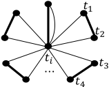
trips contain two games). The optimal itinerary graph of a

team ti may look like the graph in Figure 2.

𝑡𝑡ସ

Figure 2: the itinerary graph of team ti

Team ti must travel to or from each other team at least once, which are denoted by light lines in Figure 2. The weight sum of all light lines is ∑j̸=i Di,j = Di. The remaining dark lines in Figure 2 form a perfect matching of the graph G. Recall that we use M to denote a minimum perfect matching of G. Then the weight sum of all dark lines is at most DM. The independent lower bound for team ti is

The independent lower bound for TTP-2 is

For any team, it is possible to get its independent lower bound. The itinerary of a team is called perfect if the distance of it achieves the independent lower bound. However, not all teams may reach perfect itineraries synchronously in a feasible schedule [Thielen and Westphal, 2012]. So the independent lower bound for TTP-2 is not achievable.

𝑡𝑡ଷ

𝑡𝑡ସ

𝑢𝑢ଶ

3.2 An Upper Bound

Next, we consider a simple upper bound on the traveling distance of any feasible solution. By the triangle inequality, we can easily see that

Lemma 1. The traveling distance of any itinerary of a team ti is at most 2Di.

Lemma 1 says that the worst itinerary consisting of only road trips of one game. Lemma 1 and (1) imply that

Lemma 2. The traveling distance of any feasible itinerary of a team ti is at most the traveling distance of the optimal itinerary plus Di.

Note that Di ≤ LBi. We get that

Theorem 1. Any feasible schedule for TTP-2 is a 2approximation solution.

Indeed, Theorem 1 was first proved in [Thielen and Westphal, 2012]. We repeat this result in detail because we need to use Lemma 2 in our analysis.

4 Construction of The Tournament

To get a good theory bound and good performance, we will try to design a feasible schedule such that the itinerary of each team is similar to the perfect itinerary as much as possible.

It is not easy to find a simple feasible schedule for TTP2. Compared with known feasible schedules, our schedule is not very complicated. However, our schedule will be slightly different for n ≡ 2 (mod 8) and n ≡ 6 (mod 8). We will describe the algorithm for the case of n ≡ 2 (mod 8). For the case of n ≡ 6 (mod 8), only some edges will have different directions. These edges will be denoted by dash lines and we will explain them.

We regard each pair of teams in the minimum per-

fect matching M of G as a super-team, and first arrange

games between super-teams. There are n teams and then

there are m super-teams. We denote the super-teams as

{u1, u2, . . . , um-1, um}. We relabel the n teams such that

ui = {t2i-1, t2i} for each i. For the sake of presentation, we

will also denote ul = um-1 (resp., ur = um), and denote

the two teams in ul as {tl1, tl2} (resp., the two teams in ur as

{tr1, tr2}).

We first arrange super-games between super-teams ui and

then we will extend super-games to normal games between

normal teams ti.

Each super-team will attend m - 1 super-games in m - 1

time slots. Each super-game in the first m- 2 time slots will

be extended to four normal games between normal teams, and

each super-game in the last time slot will be extended to six

normal games between normal teams. So each normal team

ti will attend 4×(m-2)+6 = 4m-2 = 2n-2 games. This

is the number of games each team ti should attend in TTP-2.

We first design the super-games between super-teams in

the first m- 2 time slots, and then consider super-games in

the last time slot. In each of the first m- 2 time slots, we

have m-1

game involves three super-teams and all other super-games

2 super-games (note thatmis odd), where one super-

involve two super-teams. In the first slot, the m-1

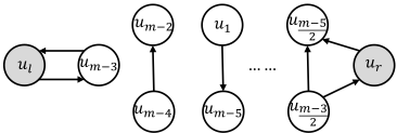
games are arranged as shown in Figure 3. The most left super-

2 super-

game involving super-team ul is called the left super-game, and the most right super-game involving ur is called the right super-game. The right super-game is the only super-game involving three super-teams. The other m-1

are called middle super-games. There are also directed edges

2 -2 super-games

in the super-games, which will be used to extend super-games

to normal games.

𝑢𝑢𝑙𝑙

𝑢𝑢𝑚𝑚-ଶ

……

𝑢𝑢𝑚𝑚-ଷ 𝑢𝑢𝑚𝑚-ସ

𝑢𝑢𝑚𝑚-ଵ

ଶ

Figure 3: Schedule at the first slot

Note that the white nodes (super-teams u1, . . . , um-2) in

Figure 3 form a cycle u1u2 . . . um-2. In the second slot,

super-games are scheduled as shown in Figure 4. we change

the positions of white super-teams in the cycle by moving one

position in the clockwise direction, and also change the direc-

tion of each edge. The positions of ul and ur will always be

fixed.

𝑢𝑢𝑟𝑟

The schedules for the first m- 2 slots are derived analo-

gously. Next, we explain how to extend the super-games in

these slots to normal games.

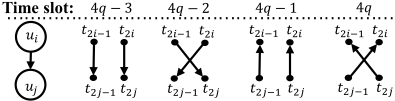
Case 1: Middle super-games. We first consider middle

super-games, each of which will be extended to four nor-

mal games in four days. Assume that in a middle super-

game, team ui plays against the team uj on time slot q,

1 ≤ i, j, q ≤ m- 2. Recall that ui represents normal teams

{t2i-1, t2i} and uj represents normal teams {t2j-1, t2j}. The

super-game will be extended to eight normal games in four

corresponding days from 4q - 3 to 4q, as shown in Figure 5.

A directed edge from team ti′ to team ti′′ means ti′ plays

against ti′′ at the home of ti′′ . Note that if there is a directed

edge from uj to ui, then the direction of all the edges in Fig-

ure 5 should be reversed.

Case 2: Left super-games. Assume that in a left supergame, team ul plays against team ui on time slot q, 1 ≤ i, q ≤ m - 2. Recall that ul represents normal teams

{t2m-3, t2m-2} and ui represents normal teams {t2i-1, t2i}.

The super-game will be extended to eight normal games in

four corresponding days from 4q - 3 to 4q, as shown in Fig-

ure 6 for odd time slot q. For even time slot q, the direction

of edges in the figure will be reversed.

𝑢𝑢𝑙𝑙

𝑢𝑢𝑖𝑖

𝑢𝑢𝑟𝑟

𝑡𝑡𝑙𝑙𝑙

𝑡𝑡ଶ𝑖𝑖

𝑡𝑡𝑙𝑙𝑙

𝑡𝑡ଶ𝑖𝑖

𝑡𝑡𝑙𝑙𝑙

𝑡𝑡ଶ𝑖𝑖

𝑡𝑡𝑙𝑙𝑙

𝑡𝑡ଶ𝑖𝑖

Figure 6: Left super-games

Case 3: Right super-games. Assume that in a right super-

game, three teams ui, ui-1 and ur play on time slot q, 1 ≤

i, q ≤ m- 2 and u0 = um-2. Recall that ur represents nor-

mal teams {t2m-1, t2m}. The super-game will be extended to

twelve normal games in four corresponding days from 4q -3

to 4q, as shown in Figure 7. Note that the edges between

three teams are dash edges (see Figures 3 and 4). So for the

case of n ≡ 6 (mod 8), the direction of these three edges

should be reversed. So Figure 7 describes the case of odd

time slot q with n ≡ 2 (mod 8) and the case of even time

slot q with n ≡ 6 (mod 8). For the case of odd time slot q

with n ≡ 2 (mod 8) and the case of even time slot q with

n ≡ 6 (mod 8), the direction of all edges in the figure will

be reversed.

Time slot:

……………………………………………………………

𝑢𝑢𝑖𝑖-ଵ

𝑢𝑢𝑖𝑖

4𝑞𝑞 - 3

𝑡𝑡ଶ𝑖𝑖-ଷ

𝑡𝑡ଶ𝑖𝑖-ଵ

𝑡𝑡ଶ𝑖𝑖

4𝑞𝑞 - 2

𝑡𝑡ଶ𝑖𝑖-ଷ

𝑡𝑡ଶ𝑖𝑖-ଵ

𝑡𝑡ଶ𝑖𝑖

4𝑞𝑞 - 1

𝑡𝑡ଶ𝑖𝑖-ଷ

𝑡𝑡ଶ𝑖𝑖-ଵ

𝑡𝑡ଶ𝑖𝑖

4𝑞𝑞

𝑡𝑡ଶ𝑖𝑖-ଷ

𝑡𝑡ଶ𝑖𝑖-ଵ

𝑡𝑡ଶ𝑖𝑖

Figure 7: Right super-games

The first m-2 slots will be extended to 4(m-2) = 2n-8

days according to the above rules. Each team will have six re-

maining games, which will be scheduled in the last time slot.

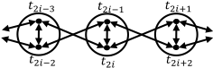
Two remaining games are self-games, which is to play against the team in the same super-team. For teams in ul and ur, the other four remaining games are between the teams in ul and ur. For teams in the other super-teams ui, two remaining

games should be played against a team in super-team ui-1

and two remaining games should be played against a team

in super-team ui+1, such as the two missing games between

t2i-3 and t2i in Figure 7. Figure 8 shows the six remaining

games for teams in ui (i ∈ {1, 2, . . . ,m- 2}), and Figure 9

shows the six remaining games for teams in ul and ur.

𝑡𝑡ଶ𝑖𝑖

𝑡𝑡ଶ𝑖𝑖+ଶ

Figure 8: The six remaining games for teams in ui (i ̸= l, r)

The last slot. Now we are ready to design the six days of games for the last slot. We use self to denote one day of selfgames: for each super-teamui, team t2i-1 plays against team

𝑡𝑡ଶ𝑖𝑖-ଶ

𝑡𝑡𝑟𝑟𝑟

𝑡𝑡𝑟𝑟𝑟

𝑡𝑡ଶ𝑖𝑖-ଶ

𝑡𝑡𝑟𝑟𝑟

𝑡𝑡𝑟𝑟𝑟

𝑡𝑡ଶ𝑖𝑖-ଶ

𝑡𝑡𝑟𝑟𝑟

𝑡𝑡𝑟𝑟𝑟

𝑡𝑡ଶ𝑖𝑖-ଶ

𝑡𝑡𝑟𝑟𝑟

𝑡𝑡𝑟𝑟𝑟

𝑡𝑡ଵ

𝑡𝑡ଶ

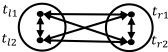
t2i at the home of t2i. We will also use self to denote the day of games with the reversed direction in self, i.e., the partner is the same but the game site change to the other team's

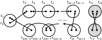
home. We also design two days of games A1 and A2 as shown

in Figures 10 and 11. Then we can see that the other four

days of games left are given by A1,A2,A1,A2. Note that in

A1, A2, A1, and A2 we will have three dash edges, which will

be reversed for the case of n ≡ 6 (mod 8).

𝑡𝑡ଷ 𝑡𝑡ସ

𝑡𝑡ହ 𝑡𝑡଺

……

𝑡𝑡ଶ𝑚𝑚-ହ 𝑡𝑡ଶ𝑚𝑚-ସ

𝑡𝑡ଶ𝑚𝑚-଻ 𝑡𝑡ଶ𝑚𝑚-଺

𝑡𝑡𝑚𝑚-ଶ 𝑡𝑡𝑚𝑚-ଵ

𝑡𝑡𝑚𝑚 𝑡𝑡𝑚𝑚+ଵ

Figure 10: The day A1

𝑡𝑡ଶ𝑚𝑚-ହ 𝑡𝑡ଶ𝑚𝑚-ସ

𝑡𝑡ଶ𝑚𝑚-଻ 𝑡𝑡ଶ𝑚𝑚-଺

𝑡𝑡𝑚𝑚 𝑡𝑡𝑚𝑚+ଵ

𝑡𝑡𝑙𝑙𝑙 𝑡𝑡𝑙𝑙𝑙

𝑡𝑡𝑟𝑟𝑟 𝑡𝑡𝑟𝑟𝑟

𝑡𝑡𝑟𝑟𝑟 𝑡𝑡𝑟𝑟𝑟

Figure 11: The day A2

Next, we need to order the six days {self, self, A1,A2, A1, A2} to joint the previous 2n-8 days without violating the bounded-by-k and no-repeat constraints. It will be different for the two cases of n ≡ 2 (mod 8) and n ≡ 6 (mod 8). For n ≡ 2 (mod 8), the six days are arranged in the order: A1, self, A2, self, A2, A1; For n ≡ 6 (mod 8), the six days are arranged in the order: A2, self , A1, self, A1, A2.

We have described the main part of the scheduling algorithm. Next, we will prove its feasibility.

Theorem 2. For TTP-2 with n teams such that n ≥ 10 and n ≡ 2 (mod 4), the above construction can generate a feasible schedule.

Proof. First, we show that each team plays all the required 2n-2 games in the 2n-2 days. According to the schedule, we can see that each team will attend one game in each of the 2n - 2 days. Furthermore, it is not hard to observe that no two teams play against each other at the same place. So each team will play the required 2n - 2 games.

Second, it is easy to see that each teamwill not violate the no-repeat property. In any time slot, no two games between the same teams are arranged in two consecutive days. For two different time slots, each team will play against different teams. Especially, self and self are not arranged as two consecutive days in the last time slot.

Last, we prove that each team does not violate the bounded-by-k property. We will use 'H' and 'A' to denote a home game and an away game, respectively. We will also let H = A and A = H.

We first look at the games in the first 2n - 8 days. For the two teams in ul, the 4 games in an odd time slot will be HAAH (see Figure 6), and the 4 games in an even time slot will be AHHA. So two consecutive time slots can be jointed well. For the two teams in ur, the 4 games will be HAAH or HAAH in an odd time slot and reversed in an even time slot. Two consecutive time slots can still be jointed well. Next, we consider a team ti in uj (j ∈ {1, 2, . . . ,m - 2}). In the time slots for middle super-games, the 4 games will be AAHH if the direction of the edge (super-game) is toward uj and AAHH otherwise. In the time slots for left supergames, the 4 games will be AHHA or AHHA. In the time slots for right super-games, the 4 games will be AAHH or AAHH. According to our schedule, two consecutive time slots can joint well, no matter they are two slots for middle super-games, or one slot for middle super-game and one slot for left super-game, or one slot for middle super-game and one slot for right super-game.

We have the last 6 days in the last time slot not analyzed yet. For the sake of presentation, we just list out the last 10 games in the last two time slots for each team. We will

have five different cases: teams in ul, ur, u1, u0 for odd

o ∈ {3, . . . ,m- 2}, and ue for even e ∈ {2, . . . ,m- 2}.

The reason why u1 is different from other uo with an odd

subscript o is that in the penultimate time slot, u1 plays with

ul, and then it has a different form of games. For the case of

n ≡ 2 (mod 8), the last 10 games are shown in Figure 12,

and for the case of n ≡ 6 (mod 8), the last 10 games are

shown in Figure 13. We can see that there are no three con-

secutive home games or away games. So the bounded-by-k

property holds.

𝑢𝑢𝑙𝑙 �𝑡𝑡𝑙𝑙𝑙: 𝐻𝐻𝐻𝐻𝐻𝐻𝐻𝐻𝐴𝐴𝐴𝐴𝐴𝐴𝐴𝐴𝐴𝐴𝐴𝐴

𝑡𝑡𝑙𝑙2: 𝐻𝐻𝐻𝐻𝐻𝐻𝐻𝐻𝐴𝐴𝐴𝐴𝐴𝐴𝐴𝐴𝐴𝐴𝐴𝐴

𝑢𝑢𝑟𝑟 �𝑡𝑡𝑟𝑟1: 𝐻𝐻𝐻𝐻𝐻𝐻𝐻𝐻 𝐻𝐻𝐻𝐻𝐻𝐻𝐻𝐻𝐻𝐻𝐻𝐻

𝑡𝑡𝑟𝑟𝑟:𝐴𝐴𝐴𝐴𝐴𝐴𝐴𝐴𝐻𝐻𝐻𝐻𝐻𝐻𝐻𝐻𝐻𝐻𝐻𝐻

𝑡𝑡𝑙𝑙2: 𝐻𝐻𝐻𝐻𝐻𝐻𝐻𝐻𝐴𝐴𝐴𝐴𝐴𝐴𝐴𝐴𝐴𝐴𝐴𝐴

𝑢𝑢1 �𝑡𝑡1:𝐴𝐴𝐴𝐴𝐴𝐴𝐴𝐴𝐻𝐻𝐻𝐻𝐻𝐻𝐻𝐻𝐻𝐻𝐻𝐻

𝑡𝑡2: 𝐴𝐴𝐴𝐴𝐴𝐴𝐴𝐴𝐴𝐴𝐴𝐴𝐴𝐴𝐴𝐴𝐴𝐴𝐴𝐴

𝑢𝑢𝑜𝑜 �𝑡𝑡𝑜𝑜𝑜: 𝐻𝐻𝐻𝐻𝐻𝐻𝐻𝐻 𝐻𝐻𝐻𝐻𝐻𝐻𝐻𝐻𝐻𝐻𝐻𝐻

𝑡𝑡𝑜𝑜𝑜: 𝐻𝐻𝐻𝐻𝐻𝐻𝐻𝐻 𝐻𝐻𝐻𝐻𝐻𝐻𝐻𝐻𝐻𝐻𝐻𝐻

𝑢𝑢𝑒𝑒 �𝑡𝑡𝑒𝑒𝑒:𝐴𝐴𝐴𝐴𝐴𝐴𝐴𝐴𝐴𝐴𝐴𝐴𝐴𝐴𝐴𝐴𝐴𝐴𝐴𝐴

𝑡𝑡𝑒𝑒𝑒: 𝐴𝐴𝐴𝐴𝐴𝐴𝐴𝐴𝐴𝐴𝐴𝐴𝐴𝐴𝐴𝐴𝐴𝐴𝐴𝐴

Figure 12: The last 10 games for the case of n ≡ 2 (mod 8)

𝑢𝑢𝑙𝑙 �𝑡𝑡𝑙𝑙𝑙: 𝐻𝐻𝐻𝐻𝐻𝐻𝐻𝐻𝐴𝐴𝐴𝐴𝐴𝐴𝐴𝐴𝐴𝐴𝐴𝐴

𝑢𝑢𝑟𝑟 �𝑡𝑡𝑟𝑟1:𝐴𝐴𝐴𝐴𝐴𝐴𝐴𝐴𝐻𝐻𝐻𝐻𝐻𝐻𝐻𝐻𝐻𝐻𝐻𝐻

𝑡𝑡𝑟𝑟𝑟: 𝐻𝐻𝐻𝐻𝐻𝐻𝐻𝐻 𝐻𝐻𝐻𝐻𝐻𝐻𝐻𝐻𝐻𝐻𝐻𝐻

𝑢𝑢1 �𝑡𝑡1:𝐴𝐴𝐴𝐴𝐴𝐴𝐴𝐴𝐴𝐴𝐴𝐴𝐴𝐴𝐴𝐴𝐴𝐴𝐻𝐻

𝑡𝑡2:𝐴𝐴𝐴𝐴𝐴𝐴𝐴𝐴𝐻𝐻𝐻𝐻𝐻𝐻𝐻𝐻𝐻𝐻𝐻𝐻

𝑢𝑢𝑜𝑜 �𝑡𝑡𝑜𝑜𝑜: 𝐻𝐻𝐻𝐻𝐻𝐻𝐻𝐻 𝐻𝐻𝐻𝐻𝐻𝐻𝐻𝐻𝐻𝐻𝐻𝐻

𝑡𝑡𝑜𝑜𝑜: 𝐻𝐻𝐻𝐻𝐻𝐻𝐻𝐻 𝐻𝐻𝐻𝐻𝐻𝐻𝐻𝐻𝐻𝐻𝐻𝐻

𝑢𝑢𝑒𝑒 �𝑡𝑡𝑒𝑒𝑒:𝐴𝐴𝐴𝐴𝐴𝐴𝐴𝐴𝐴𝐴𝐴𝐴𝐴𝐴𝐴𝐴𝐴𝐴𝐴𝐴

𝑡𝑡𝑒𝑒𝑒: 𝐴𝐴𝐴𝐴𝐴𝐴𝐴𝐴𝐴𝐴𝐴𝐴𝐴𝐴𝐴𝐴𝐴𝐴𝐴𝐴

Figure 13: The last 10 games for the case of n ≡ 6 (mod 8)

Since our schedule satisfies the above three conditions, we

know that our schedule is a feasible schedule for TTP-2. Note

that our schedule requires at least 10 teams. So we have n ≥

10.

5 Analyzing Approximation Quality

Next, we analyze the theoretical approximation bound of our schedule. We compare the itinerary of each team in our schedule with the perfect itinerary and use ∆i to denote the difference between them for each team i. Then we only need to evaluate a bound for ∑ni=1 ∆i.

We first introduce the framework of our proof idea. For team ti with 1 ≤ i ≤ n - 4 in a white super-team uj in Figure 3, only its trips to the nine teams in ul ∪ ur ∪ uj-1 ∪ uj ∪ uj+1 \ {ti} may be different from that in the perfect itinerary. By Lemma 2, we know that the distance of this part in our schedule will be at most that in the perfect itinerary plus the nine distances from ti to the nine teams. On average, each team ti will use an extra distance of about 9/n of the independent low bound LBi. For teams ti (i ∈ {1, 2, . . . , n4}), the total extra distance will be bounded by about 9/n of LB. For the other four teams ti (i ∈ {n-3, n-2, n-1, n}) in the two super-teams ul and ur, their itineraries may be totally different from the perfect itineraries. However, by Lemma 2, we know that the extra distance for ti is most LBi. We will set the four teams with the minimum value LBi. Then the extra distance given by the four teams is at most 4/n of LB. Thus, we get an approximation ratio of about (1 + 13/n). Next, we give a more detailed analysis and show a refined ratio of (1 + 12/n) indeed.

First, we consider the four teams {tn-3, tn-2, tn-1, tn} in

the two super-teams ul and ur. By Lemma 2, we directly get

that∆i ≤ LBi for each i ∈ {n-3, n-2, n-1, n}.

(3)

Second, we consider the n - 4 teams ti in super-teams uj

(j ∈ {1, 2, . . . ,m - 2}). We look at two super-teams ui1

and ui2 , where 1 ≤ i1, i2 ≤ m- 2 and |i1 - i2| ≥ 2. The

games between the two super-teams will be the form of mid-

dle super-games in Case 1. A team in ui1 (resp., ui2 ) will

visit the two teams in ui2 (resp., ui1 ) in one road trip, which

is also a road trip in the perfect itinerary. Comparing with the

perfect itinerary for a team ti ∈ uj (i ∈ {1, 2, . . . , n - 4},

and j = ⌈i/2⌉), only the trips to visit the nine teams in

ul ∪ ur ∪ uj-1 ∪ uj ∪ uj+1 \ {ti} may be different. See

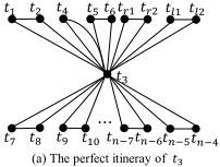
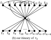
the comparison for t3 as an example in Figure 14.

(a) The perfect itineray of 𝑡𝑡ଷ

(b) our itineary of 𝑡𝑡ଷ

Figure 14: The perfect itinerary and our itinerary of t3: the lower parts are the same and the upper parts of the trips to the nine teams are different

By Lemma 2, we know that

Claim. For each ti ∈ uj (i ∈ {1, 2, . . . , n - 4}, and j = ⌈i/2⌉), ∆i is bounded by the sum of the distances from ti to the nine teams in ul ∪ ur ∪ uj-1 ∪ uj ∪ uj+1 \ {ti}.

Recall that for two super-games ui and uj, we use D(ui, uj) to denote the sum of the four distances between teams tp ∈ ui and tq ∈ uj. By the above claim, we get that

where u0 is interpreted as um-2.

Next, we reorder the teams to get good bounds for B1 = ∑ni=n-3 LBi and B2 = ∑m-2 i=1 D(ui-1, ui). Since LB = ∑mi=1 (LB2i-1 +LB2i), we can choose ul and ur such that

Next, we choose an order of ui to make B2 as small as possible. Recall that H is the complete graph on the m super-teams ui. We decompose the complete graph H into (m - 1)/2 edge-disjoint Hamilton cycles by using the wellknown decomposition algorithm in [Alspach et al., 1990] and let C be one Hamilton cycle among them having the minimum length. Then we reorder ui such that u1u2 . . . um-2 is a part of the Hamilton cycle C. Therefore, by the triangle inequality, we get

By (3)-(6), we get that

Theorem 3. There is a polynomial-time (1 + 8n + 4 n-2 )- approximation algorithm for TTP-2 with n teams, where n ≥ 10 and n ≡ 2 (mod 4).

6 Experimentations

To test the experimental performance, we will also use one more local-search trick. Note that after getting a feasible schedule by the above algorithm, we can get more feasible schedules by only changing the positions of the teams. In the experiments, we use two local-search rules to check better solutions: swap between two super-teams and swap between two teams in each super-team. This will lead O(m3 ) loops, and then the running-time bound will increase a factor of m3 .

We implement our algorithm to solve the benchmark instances in [Trick, 2021]. The website introduces 62 instances, most of which were reported from real-world sports scheduling scenarios, such as the Super 14 Rugby League, the National Football League, and the 2003 Brazilian soccer championship. The number of teams in the instances varies from 4 to 40. We can solve all the 23 instances of n teams with n ≥ 10 and n ≡ 2 (mod 4), in which 7 instances are very special (all teams are in a cycle or all distance between pairs of teams are 1) and not tested in previous papers. For the remaining 16 instances, we compare our results with the bestknown results in Table 1. In the table, the column 'Lower Bound' indicates the independent lower bounds, 'Previous Results' lists previous known results in [Thielen and Westphal, 2012], 'Our Results' shows the results given by our schedule algorithm after local search, and 'Improvement Ratio' is defined as Previous Results - Our Results Previous Results .

Table 1: Experimental results

Data Sets	Lower Bounds	Previous Results	Our Results	Improvement Ratio(%)
Galaxy38	244848	274672	262657	4.37
Galaxy34	173312	192317	185347	3.62
Galaxy30	113818	124011	122628	1.12
Galaxy26	68826	77082	75538	2.00
Galaxy22	40528	46451	45360	2.35
Galaxy18	23774	27967	27467	1.79
Galaxy14	12950	15642	15622	0.13
Galaxy10	5280	6579	6506	1.11
NFL30	951608	1081969	1038902	3.98
NFL26	669782	779895	745595	4.40
NFL22	504512	600822	574028	4.46
NFL18	361204	439152	423326	3.60
NL14	238796	296403	289323	2.39
NL10	70866	90254	87842	2.67
Super14	823778	1087749	1019941	6.23
Super10	392774	579862	589512	-1.66

From this table, we can see that our scheduling improves 15 out of 16 instances. The average improvement on the 16 instances is 2.66%. Our algorithm is also fast. On a standard laptop with a 2.30GHz Intel(R) Core(TM) i5-6200 CPU and 8 GB RAM, all the 16 instances can be solved together within 0.1 seconds before applying local search and within 30 seconds including local search.

7 Conclusion

We have designed an algorithm to generate a feasible solution to TTP-2 with n ≡ 2 (mod 4), which can guarantee the traveling distance at most (1 + 8n + 4 n-2 ) times of the optimal. This is the first (1 + O( 1n ))-approximation algorithm for TTP-2 with n ≡ 2 (mod 4). The algorithm is also very practical. Experimental results show that our algorithm can beat best-known solutions for almost all instances with n ≥ 10 and n ≡ 2 (mod 4) in the well-known benchmark. Furthermore, we are able to get further improvements by using a simple local-search method. In the experiments, we only consider exchanges between two teams (or super-teams) each time. We may be able to get more improvements by considering exchanges among three or more teams. However, the running time will increase dramatically and the improvement is very limited.

Acknowledgments

The work is supported by the National Natural Science Foundation of China, under grants 61972070.