On Weak Stubborn Sets in Classical Planning

1 Introduction

Planning as search is a leading approach to optimal domainindependent planning. As the induced search spaces generally grow exponentially in the size of the compact planning problem description, additional pruning functions are desired to cut down the search space's size. Pruning functions are supposed to retain at least one (optimal) solution.

Stubborn sets have been introduced as a pruning function for model checking Petri nets [Valmari, 1989], in the form of strong and weak stubborn sets. In the last decade, stubborn sets have also been investigated for AI planning in various ways [Wehrle and Helmert, 2012; Alkhazraji et al., 2012; Wehrle et al., 2013; Wehrle and Helmert, 2014; Winterer et al., 2017; Al-Khazraji, 2017; Keren et al., 2018; Wilhelm et al., 2018; Schulte, 2018; Gnad et al., 2019; R¨oger et al., 2020]. As pointed out by Valmari in his original work, weak stubborn sets potentially allow for more pruning than their strong counterpart. However, while the strong version has been considered rather extensively, weak stubborn sets have hardly been analyzed for AI planning so far.

In this work, we revisit weak stubborn sets for planning. We show that recently discussed pruning functions called weak stubborn sets for planning [Winterer et al., 2017; Al-Khazraji, 2017; Wilhelm et al., 2018] are actually not weak stubborn sets in the formal sense as introduced by Valmari [1989]. Motivated by this finding, we introduce weak stubborn sets in Valmari's sense for classical planning. We define them as generalized weak stubborn sets, analogously to generalized strong stubborn sets [Wehrle and Helmert, 2014], and investigate their relationship to existing stubborn set approaches. Altogether, our work provides a further step in getting an overall picture and understanding of the stubborn set approach in AI planning.

2 Preliminaries

We consider optimal SAS+ planning, where states of the world are represented based on a finite set of finite-domain variables V. Every variable v ∈ V has a finite domain D(v). For a subset P ⊆ V, a partial state s is defined as a function s : P → D(P) that maps the variables in P to the domain of their variables, where D(P) is defined as ∪v∈PD(v). We say that s is defined on variables in P. For all remaining variables V \ P that are not contained in P, the partial state s is undefined. In the special case where s is defined on all variables in V, we call s a state. A variable/value assignment {v ↦→ p} is called a fact. For a partial state s and fact {v ↦→ p}, we will sometimes use the notation s |= {v ↦→ p} to denote that v has value p in s. Furthermore, for partial states s and s′ and a variable v, we say that s and s′ match on v iff s(v) and s(v′ ) are defined, and s(v) = s′ (v). We say that s satisfies s′ if s and s′ match on all variables where s′ is defined.

States are changed with operators o = 〈pre(o), eff (o)〉, where pre(o) and eff (o) are partial states. Every operator o has an associate non-negative cost cost(o) ∈ R+0 . An operator o is applicable in state s iff s satisfies pre(o). In this case, the application of o in s yields the successor state o(s), where o(s) is obtained from s by changing the values of all variables in s such that o(s) satisfies eff (o) and retains the values of the variables in s where eff (o) is undefined. For a state s, the set of applicable operators in s is denoted with app(s).

A planning task Π = (V,O, s0, s⋆) is defined as a tuple consisting of a finite set of finite-domain variables V, a finite set of operators O, an initial state s0 and a partial goal state s⋆. A sequence π of operators which is iteratively applicable starting in a state s and which leads to a state s′ such that s′ satisfies the partial goal state is called a plan for s. A plan for Π is a plan for s0 of Π. States for which a plan exists are called solvable, other states are called unsolvable. The cost of a plan is the summed costs of each operator of the sequence. A plan π for s is called optimal if its cost is minimal among all plans for s. A plan π for s is called strongly optimal if π is optimal for s and contains a minimal number of zero-cost operators among all optimal plans for s. Our objective is to find an optimal plan for Π.

2.1 Safe Pruning with Stubborn Sets

We consider planning as search using safe pruning functions that restrict the successors of a state s to subsets of app(s) as introduced by Wehrle and Helmert [2014]. A pruning function is called safe if for every state s, the costs of an optimal plan for s in the pruned state space and in the original state space are the same.

As a basis for the paper, we provide the notions of generalized strong stubborn sets. Stubborn sets crucially rely on the notion of interference. In previous work, interference has been defined both in a state-based fashion [e.g., Wehrle and Helmert, 2014], as well as in a syntax-based fashion as an approximation thereof [e.g., Alkhazraji et al., 2012]. As the differentiation will be crucial for the analyses in the following, we will introduce both the state-based notions (now) and syntactic-based notions (later in the paper), using the naming convention to leave out the name "state-based" for brevity. We start by giving the definition of disabling operators and interference according to Wehrle and Helmert [2014].

Definition 1 (disabling, conflicting). Let o1 and o2 be operators of a planning task Π, let s be a state of Π, and let o1 and o2 be both applicable in s. Then we say that

• o1 disables o2 in s if o2 /∈ app(o1(s)).
• o1 disables o2 on fact {v ↦→ p} in s if pre(o2) |= {v ↦→ p} and o1(s) ̸|= {v ↦→ p}.
• o1 and o2 conflict in s if s12 = o2(o1(s)) and s21 = o1(o2(s)) are both defined and differ (i.e., s12 ̸= s21).

Two operators interfere in a state if they cannot be executed in both possible orderings, leading to the same state. We distinguish interference and weak interference.

Definition 2 (interference). Let o1, o2 be operators of a planning task Π, and let s be a state of Π. We say that o1 weakly interferes with o2 in s if they are both applicable in s, and

• o1 disables o2 in s, or
• o1 and o2 conflict in s.

Furthermore, we say that o1 interferes with o2 in s if they are both applicable in s, and

• o1 weakly interferes with o2 in s, or
• o2 disables o1 in s.

The differentiation of weak interference and interference will be important for the differentiation of strong and weak stubborn sets. We observe that the notion of interference is symmetric (conflict is a symmetric notion and two operators interfere if one disables the other, no matter the direction), but that this is not the case for weak interference (i.e., o1 can weakly interfere with o2 in a state s, while o2 does not necessarily weakly interfere with o1 in s). Also note that weak interference implies interference.

Furthermore, for the definition of generalized strong stubborn sets, we need the notion of necessary enabling sets.

Definition 3 (necessary enabling set, Wehrle and Helmert 2014). Let Π be a planning task, let o be an operator of Π, and let Seq be a set of operator sequences applicable in the initial state of Π. A necessary enabling set for o and Seq is a set N of operators such that every operator sequence in Seq which includes o as one of its operators also includes an operator o′ ∈ N before the first occurrence of o.

We now provide the conditions needed for generalized strong stubborn sets, introduced by Wehrle and Helmert [2014]. For a planning task Π = (V,O, s0, s⋆), a solvable state s in Π, and an associated envelope E ⊆ O, we define the task ΠEs = (V, E, s, s⋆). 1 For such a task ΠEs , we define Opt as the set of strongly optimal plans for ΠEs , and SOpt as the set of states that are visited by at least one strongly optimal plan in Opt. Let T ⊆ O be a set of operators. We define the following conditions for E and T :

• C1: E includes all operators from at least one strongly optimal plan for s (in task Π).
• C2: T contains at least one operator from at least one strongly optimal plan for ΠEs .
• C3: For every o ∈ T not applicable in s, T contains a necessary enabling set for o and Opt .
• C4: For every o ∈ T applicable in s, T contains all operators o′ ∈ E such that o′ interferes with o in any state s′ ∈ SOpt .

We can now define generalized strong stubborn sets.

Definition 4 (generalized strong stubborn set, Wehrle and Helmert 2014). Let Π = (V,O, s0, s⋆) be a planning task, E an associated envelope, and s a state of Π. A generalized strong stubborn set (GSSS) in s is a set of operators T ⊆ O with the following properties. If s is an unsolvable state or a goal state, every set T ⊆ O is a GSSS in s. If s is a solvable non-goal state, then T is a GSSS in s if conditions C1, C2, C3 and C4 are true for E and T .

Applying only the operators from a GSSS in a state s guarantees that for at least one strongly optimal plan π in s, there is a permutation π′ of π such that π′ is not pruned in s and π′ is a plan in s. Hence, GSSS yield safe pruning functions.

As computing the interference relationship effectively relies on computing the set of states in SOpt , which is computationally as hard as solving the planning task itself, this computation has been approximated in practice. A simple approximation is checking the interference based on the pure operator syntax (we will come back to this in the next section). A more sophisticated approximation for both SOpt and the operator interference relation is to use mutex-based interference. Two facts f and f ′ are called mutex if no reachable state satisfies both f and f ′ [Bonet and Geffner, 2001]. While the general computation of mutexes is as hard as solving the original planning task, there exist sound but incomplete polynomial-time algorithms to compute mutexes up to a fixed size [e.g., Rintanen, 2008; Helmert, 2009]. Two operators o and o′ are called mutex if there exists a pair of facts

1 Wehrle and Helmert [2014] characterize an envelope as "an operator set that is known to be sufficient in the sense that we can safely treat all operators outside the envelope as if they did not exist".

(f, f ′ ) such that f and f ′ are mutex, f is contained in the precondition of o, and f ′ is contained in the precondition of o′ . For mutex operators, we know that there is no reachable state where both of them are applicable, hence in particular they do not interfere in any state in SOpt .

3 The Operator Shifting Property

In his original work, Valmari [1989] stated that stubborn sets T in a state s remain stubborn sets in the successor state o(s) if o is not contained in T (see Theorem 1.19 in his paper). While this stubborn property holds for strong and weak stubborn sets, it does no longer hold for GSSS, as GSSS restrict the consideration to preserve only at least one strongly optimal plan (instead of preserving a permutation of every plan) for s: If there are strongly optimal plans π1 and π2 for s, and a GSSS T only contains operators in π1, then T does not need to be a GSSS in o(s) if o is the first operator of π2. 2

In the following, we focus on a slightly more general property to characterize stubborn sets, which reflects the original key idea of stubborn sets on the one hand, but abstracts away from the set of plans that are preserved. We call this property "operator shifting property".

Definition 5 (operator shifting property). Let Π be a planning task, s be a state of Π and T be a subset of the operators of Π. We say that T has the operator shifting property in s if for all plans π = o1 . . . on for s with {o1, . . . , on} ∩ T ̸= ∅, the following holds, assuming oi to be the operator with minimal index that is contained in T (i.e., o1, . . . oi-1 ̸∈ T):

1. oi can be shifted to the front of π, i.e., π′ = oio1 . . . oi-1oi+1 . . . on is a plan, and
2. oi is also applicable in all intermediate states oj(. . . (o1(s)) . . . ) for j = 1, . . . , i - 1.

Valmari [1989] already showed in the derivation of stubborn sets that this property holds for both strong and weak stubborn sets. Later on, Wehrle and Helmert [2014] showed in the safety proof of GSSS that the operator shifting property also holds for GSSS. However, as we will see in the following, the recently considered pruning techniques in planning which have been called weak stubborn sets, including the approaches by Winterer et al. [2017], Al-Khazraji [2017], and Wilhelm et al. [2018], do not satisfy (the second part of) the operator shifting property. All of these recent techniques use notions of interference solely based on syntactically checking preconditions and effects of operators. We restate their definitions in the following.

2 To see this, consider the planning task with initial state s0 = {vi ↦→ 0} ∪ {G ↦→ 0} for 1 ≤ i ≤ 6, goal s⋆ = {G ↦→ 1}, and operators oi with pre(oi) = {vi ↦→ 0} and eff (oi) = {vi ↦→ 1} for i = 1, . . . , 4, and operators o5 and o6 with pre(o5) = {v1 ↦→ 1, v2 ↦→ 1}, pre(o6) = {v3 ↦→ 1, v4 ↦→ 1} and eff (oj) = {G ↦→ 1} for j = 5, 6, all with costs of 1. Note that we generally use upper case letters to denote variables mentioned in the goal. In s0, one can choose to use o1, o2 and o5 or alternatively o3, o4 and o6 to optimally achieve the goal. For example, T = {o1} is a GSSS in s0 because it contains an operator from a strongly optimal plan for s0, and all interfering operators are contained as well (as there are none of those). However, as o3 starts a strongly optimal plan in s0 as well, T is no longer a GSSS in s′ := o3(s0) because o1, o2, o5 yield a plan of higher cost for s′ than o4, o6 (and hence, T does not contain an operator from a strongly optimal for s′ ).

Definition 6 (syntactic weak interference). Let o1, o2 be operators of a planning task Π. We say that o1 syntactically weakly interferes with o2 if there are facts f1 = {v ↦→ p} and f2 = {v ↦→ p′ } with p ̸= p′ such that eff (o1) |= f1 and

• pre(o2) |= f2, or
• eff (o2) |= f2.

Furthermore, o1 syntactically interferes with o2 if it syntactically weakly interferes with o2 or eff (o2) |= f2 and pre(o1) |= f1.

Using interference approximations like Def. 6 is sound because every superset of interference relations still yields a safe pruning function, to the expense of less pruning power. For our later analysis, we restate the definition of weak stubborn sets along the lines of the definition used by Winterer et al. [2017], Al-Khazraji [2017], Wilhelm et al. [2018]. As we will see that these sets are not weak stubborn sets in the sense of Valmari, we redefine their name and call them "compliant stubborn sets" in the following. The definition needs the further notion of disjunctive action landmarks for a state s [Helmert and Domshlak, 2009], i.e., sets of operators L such that every plan for s contains at least one operator in L.

Definition 7 (compliant stubborn sets). Let Π = (V,O, s0, s⋆) be a planning task, and let s be a state of Π. A compliant stubborn set (CSS) in s is a set of operators T ⊆ O with the following properties. If s is an unsolvable state or a goal state, every set T ⊆ O is a CSS in s. If s is a solvable non-goal state, then the following conditions must be true for T to be a CSS in s:

1. T contains a disjunctive action landmark for s.
2. For every o ∈ T that is not applicable in s, T contains a necessary enabling set for o and the set of all applicable operator sequences in s.
3. For every o ∈ T that is applicable in s, T contains all operators o′ such that o syntactically weakly interferes with o′ .

In contrast to GSSS, the condition for applicable operators is simplified to syntactic weak interference. As pointed out in the literature, CSS yield safe pruning functions. However, they do not satisfy the operator shifting property.

Theorem 1. Compliant stubborn sets do not satisfy the operator shifting property.

Proof. We provide an example to show that Def. 5 is not satisfied. Consider the planning task with initial state s0 = {v ↦→ 0,X ↦→ 0, Y ↦→ 0,Z ↦→ 0}, goal s⋆ = {X ↦→ 1, Y ↦→ 1, Z ↦→ 1}, and operators o1, o2, o3 (cost = 1) with

• pre(o1) = {v ↦→ 0}, eff (o1) = {v ↦→ 1, X ↦→ 1}
• pre(o2) = {v ↦→ 1}, eff (o2) = {v ↦→ 0, Y ↦→ 1}
• pre(o3) = {v ↦→ 0}, eff (o3) = {Z ↦→ 1}

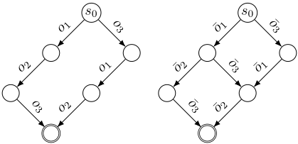
The set T = {o3} is a CSS in s0: T is a disjunctive action landmark in s0 and the only applicable operator o3 does not syntactically weakly interfere with o1 or o2. Hence neither o1 nor o2 needs to be included in T .

We observe that there are two plans for s0, namely π1 = o1o2o3 and π2 = o3o1o2, as illustrated in the left part of Fig. 1. T does not satisfy the operator shifting property in s0 because condition 2. of Def. 5 is not satisfied for π1: Although o3 can be shifted to the front, yielding the plan π2, o3 is not applicable in the intermediate state o1(s0).

The example in the proof of Theorem 1 illustrates a key difference of stubborn sets and compliant stubborn sets: Stubborn sets satisfy the operator shifting property, yielding a state space as shown in the right part of Fig. 1. In contrast, compliant stubborn sets only allow applying operators from T in certain (but generally not all) intermediate states, as there can be "blocks" of operators that (temporarily) disallow applying operators from T within such a block, yielding a state space as shown in the left part of Fig. 1.

From a more technical point of view, the operator shifting property does not hold for CSS because for applicable operators in a CSS, the only requirement to include additional operators is syntactic weak interference (see bullet point 3 in Def. 7). To reflect the original idea of weak stubborn sets in Valmari's sense, additional operators need to be included in this case [1989]. The definition of (generalized) weak stubborn sets addresses this point.

4 GeneralizedWeak Stubborn Sets

Motivated by the results of the previous section, we formally adapt Valmari's weak stubborn sets for classical planning in the following. We provide a generalized version thereof, analogously to the generalization of strong stubborn sets [Wehrle and Helmert, 2014]. For the definition of generalized weak stubborn sets, we additionally need the notion of enabling.

Definition 8 (enabling). Let o1 and o2 be operators of a planning task Π, let s be a state of Π. Let o1 be applicable in s, and o2 be not applicable in s. Then we say that

• o1 enables o2 in s if o2 ∈ app(o1(s)).
• o1 enables o2 on fact {v ↦→ p} in s if s ̸|= {v ↦→ p}, o1(s) |= {v ↦→ p}, and pre(o2) |= {v ↦→ p}.

Note that enabling o on a precondition fact p in s is a "local" property in the sense that there is no conclusion on the applicability of o in s (in contrast to disabling o on p in s).

In the following definition of generalized weak stubborn sets, we refer to conditions C1-C3 stated in Section 2.

Definition 9 (generalized weak stubborn set). Let Π = (V, O, s0, s⋆) be a planning task, E an associated envelope, and s a state of Π. A generalized weak stubborn set (GWSS) in s is a set of operators T ⊆ O with the following properties. If s is an unsolvable state or a goal state, every set T ⊆ O is a GWSS in s. If s is a solvable non-goal state, then T is a GWSS in s if conditions C1, C2, C3 and the following C4' are true for E and T .

• C4': For all o ∈ T applicable in s, T contains all o′ ∈ E such that o weakly interferes with o′ in any state s′ ∈ SOpt . Additionally, for all {v ↦→ p} with pre(o) |= {v ↦→ p}:
• T contains all operators o′ such that o′ disables o on fact {v ↦→ p} in any state s′ ∈ SOpt , or
• T contains all operators o′ such that o′ enables o on fact {v ↦→ p} in any state s′ ∈ SOpt .

The central difference to GSSS is that GWSS T allow for a relaxed constraint on the applicable operators in T, i.e., they generalize condition C4 to C4': C4' considers weak interference instead of interference and additionally requires, for every precondition fact p of an applicable operator in T, that T contains either all "disablers" of p or all "enablers" of p. Always including all disablers yields GSSS (C4' = C4 in this case) because including disabling operators means including interfering operators. Alternatively, GWSS also allow including all enablers of p instead.

We remark that in contrast to the definition of GSSS, which is purely based on the semantics of the planning task, the definition of GWSS additionally relies on a fact-based, and thus syntax-based, notion of enabling and disabling (cf. Def. 8). While defining GWSS purely based on the semantics would be possible by using only the state-based notion of enabling and disabling, such a definition would no longer allow for including both enablers and disablers for different precondition facts of the same operator, thus resulting in a less general definition. As the original definition of weak stubborn sets by Valmari [1989] already allowed choosing enablers or disablers on a fact basis, we define GWSS in the same style.

The correctness proof for GWSS works analogously to the corresponding proof for GSSS [Wehrle and Helmert, 2014].

Theorem 2. Let T be a GWSS in s. Then the successor pruning function defined as succ(s) := T ∩ app(s) is safe.

Proof. Let s be a solvable non-goal state and T be a GWSS in s. With the same proof arguments of Wehrle and Helmert, due to C1, strongly optimal plans for ΠEs are also strongly optimal for state s in Π. Hence it suffices to show that T contains the first operator of a strongly optimal plan for ΠEs .

Consider a strongly optimal plan π = o1, . . . , on for ΠEs where at least one of π's operators is also contained in T. Such a plan must exist because of C2. Let k ∈ {1, . . . , n} be the minimal index for which ok ∈ T, and let s0 , . . . , sn be the sequence of states that are visited by π, such that s0 = s, and si = oi(si-1 ) for all 1 ≤ i ≤ n. Using the same proof arguments as Wehrle and Helmert, we observe the following:

• The states s0 , . . . , sn are contained in SOpt because π is strongly optimal.

• The operator ok is applicable in s: Otherwise, because of C3, T would contain a necessary enabling set N for ok and Opt . By the definition of necessary enabling sets and because π ∈ Opt , π would include an operator from N before ok, thus contradicting the minimality of ok.
• The operator ok does not weakly interfere with any of the operators o1, . . . , ok-1 in any of the states sj for 0 ≤ j ≤ k - 1: Otherwise, the weakly interfering operators would be contained in T because of C4' with o = ok, which would contradict the minimality of k.

We show that if ok is not already the first operator in π (i.e., for k > 1), it can be shifted to the front of π. We already know that ok is applicable in s0 , and that o1 is applicable in s0 (otherwise π would not be applicable in s).

We observe that ok must also be applicable in s1 : Assume the opposite, i.e., assume o1 disables ok in s0 . According to C4', as ok is applicable in s = s0 , for all precondition facts p of ok, either all disablers or all enablers for p in some state in SOpt are contained in T , hence in particular all disablers or enablers for p in states s0 , . . . , sk-1 .

• Case "all disablers in T": If all disablers of p (in particular in s0 ) are contained in T, then T must contain o1, contradicting the minimality of k. Hence in this case, o1 cannot disable ok.
• Case "all enablers in T": If o1 disables ok in s0 , then o1 disables ok on some precondition fact p in s0 . As ok is applicable in sk-1 (because ok is part of π), it follows that there must be an operator among o2, . . . , ok-1 that enables ok on p again in some state s2 , . . . , sk-2 (otherwise ok would not be applicable in sk-1 in π). However, as all enablers of p in states s1 , . . . , sk-2 are already contained in T , this contradicts the minimality of k.

Overall, we observe that ok is applicable in s1 . With the same proof arguments of Wehrle and Helmert, this argument can be repeated to show that ok-1 and ok can be swapped in π, still yielding a valid plan because ok does not weakly interfere with ok-1. Finally, this argument in turn can be repeated to swap ok to position k - 2, k - 3, . . . , until we get the plan π′ = ok, o1, . . . , ok-1, ok+1, . . . , on. We observe that π′ is a permutation of π for which the first operator is contained in T . This concludes the proof.

The main difference to the proof of Wehrle and Helmert is the argument why ok can be shifted to the front of π, still being applicable in all intermediate states s1 , . . . , sk-1 . Informally, if applicable in s0 , then ok must stay enabled because it cannot be disabled, either because all disablers are already contained in T, or if ok were disabled, then it could not be enabled once again because all enablers are contained in T. Hence it is not possible that ok gets disabled and then enabled again later in s1 , . . . , sk-1 . In particular, this means that T satisfies the operator shifting property in s (Def. 5).

We conclude the section with the following result.

Theorem 3. The pruning power of GWSS is exponentially higher than the pruning power of GSSS.

Proof. We extend Example 2 by Al-Khazraji [2017, Section 4.1.2] which applies for CSS but not directly for GWSS.

For n ≥ 1, consider the planning task with variables V = {x, y,G1,G2} ∪ {vi | 1 ≤ i ≤ n}, initial state s0 = {V ↦→ 0 | V ∈ V}, goal s⋆ = {G1 ↦→ 1,G2 ↦→ 1}, and operators o1, o2, o3, ˆ oi, ˆ o′i for 1 ≤ i ≤ n (cost = 1) with

• pre(o1) = {x ↦→ 0}, eff (o1) = {G1 ↦→ 1}
• pre(o2) = {x ↦→ 0}, eff (o2) = {G2 ↦→ 1}
• pre(o3) = {x ↦→ 0}, eff (o3) = {x ↦→ 1, y ↦→ 1}
• pre(ˆ oi) = {vi ↦→ 0}, eff (ˆ oi) = {y ↦→ 1, vi ↦→ 1}
• pre(ˆ o′i ) = {vi ↦→ 1}, eff (ˆ o′i ) = {y ↦→ 0, vi ↦→ 0}.

For both GWSS and GSSS, we use envelopes containing all operators to satisfy C1 and we use disjunctive action landmarks to satisfy C2.

In s0, both T1 = {o1} and T2 = {o2} are disjunctive action landmarks. We argue that both T1 and T2 already satisfy the conditions of being GWSS in s0: o1 and o2 are applicable in s0 and thus, to satisfy C4', we need to include all operators o such that o1 or o2 weakly interfere with o. However, neither o1 nor o2 conflict with or disable any other operator in the task. Furthermore, we can choose to include all enablers (rather than all disables) of the precondition {x ↦→ 0} of o1 and o2. As there are no such enablers, we do not need to include any further operators and we conclude that both T1 and T2 are GWSS in s0. The pruned state space with either of these GWSS contains 3 states (assuming no successors of goal states are considered): s0, one intermediate state where either G1 or G2 is set to 1 depending on using T1 or T2, and a goal state where both G1 and G2 are set to 1.

In contrast, GSSS do not allow the option to include the enablers, but require including all disablers of {x ↦→ 0} instead: Recall that C4, in contrast to C4', requires including all operators o which interfere with o1 or o2, which translates to including all operators o which disable o1 and o2 in any state, or, in other words, for any precondition of o1 and o2. (There are no operators conflicting with o1 or o2, and if there were, they would need to be included in the case of GWSS, too.) Therefore, any GSSS T in s0 must not only include o1 or o2, but also include o3 because o3 disables o1 and o2 in s0 on {x ↦→ 0}. This directly leads to the inclusion of o1 or o2, depending on which of both we start with. Furthermore, since o3 is applicable in s0, T must also include ˆ o′i for 1 ≤ i ≤ n because they conflict with o3. As the operators ˆ o′i are not applicable in s0, T must also include necessary enabling sets for them: since every operator ˆ oi is a necessary enabling set for ˆ o′i for 1 ≤ i ≤ n due to its effect vi ↦→ 1, T also includes all ˆ oi. As a consequence, T contains all operators and there is no pruning obtained. Since ˆ oi and ˆ o′i can be applied in any permutation of 〈1, . . . , n〉, leading to different intermediate states, the state space of the task grows exponentially in n. Thus GSSS generate a state space exponentially larger than GWSS, concluding the proof.

5 Relationship To Compliant Stubborn Sets

We analyze the relationship of GWSS and CSS. Although having similar flavors, GWSS and CSS have orthogonal properties (called R1 and R2 in the following), which influence their pruning power, i.e., how much they can prune the set of applicable operators in a state.

• R1: CSS are stricter than GWSS: CSS can only be applied with syntactic, not with state-based interference. This has already been noted by Winterer et al. [2017].
• R2: CSS are less restrictive than GWSS: CSS do not satisfy the operator shifting property, as operators in a CSS need not be applicable in all intermediate states of operator sequences (recall the left part of Fig. 1).

In the following, we consider the pruning power of GWSS and CSS more closely. For the special case when GWSS are applied using the syntactic interference relation for C4' like CSS, the same disjunctive action landmarks as CSS, and full envelopes, CSS yield subsets compared to GWSS because GWSS include the same operators as CSS but additionally enablers or disablers of applicable operators to satisfy C4'. Hence, CSS have a higher pruning power in this case.

In contrast, in the general case when GWSS are applied with state-dependent interference relations (which cannot be done for CSS), there is no dominance relation.

Theorem 4. GWSS and CSS are incomparable in terms of pruning power.

Proof. To see that CSS can yield more pruning than GWSS, consider again the example in the proof of Theorem 1. As we have already seen there, T = {o3} is a CSS in s0 because T is a disjunctive action landmark in s0 and o3 does not syntactically weakly interfere with o1 or o2. Therefore, the state space when using T consists of the linear chain of the following 4 states, which we denote in the format 〈v,X, Y, Z〉: 〈0, 0, 0, 0〉, 〈0, 0, 0, 1〉, 〈1, 1, 0, 1〉, 〈0, 1, 1, 1〉.

In contrast, we show that every GWSS T in s0, using the full envelope E = {o1, o2, o3}, contains at least both applicable operators o1 and o3. We observe that all three operators are necessary in any strongly optimal plan. If we choose o1 to satisfy C2, we must include o3 because o1 disables o3 in s0 and therefore weakly interferes with it. If, however, we choose o3 to satisfy C2, there are no operators with which o3 weakly interferes, but we must either include all enablers or disablers of its precondition {v ↦→ 0}. If we choose all disablers, we have to include o1 and we are done. Otherwise, if we choose all enablers, we have to include o2. Since o2 is not applicable in s0, we have to include o1 as a necessary enabling set for o2 and the set of all operators. We conclude by observing that using the minimal GWSS T = {o1, o3} in s0 yields a state space that additionally contains the states 〈1, 1, 0, 0〉, 〈0, 1, 1, 0〉 and 〈1, 1, 1, 0〉 compared to CSS.

To see that GWSS can yield more pruning than CSS, consider the planning task with initial state s0 = {v ↦→ 0,w ↦→ 0,G1 ↦→ 0,G2 ↦→ 0}, goal s⋆ = {G1 ↦→ 1,G2 ↦→ 1}, and operators O = {o1, o2, o3} (cost = 1) with

• pre(o1) = {v ↦→ 0}, eff (o1) = {w ↦→ 1, G1 ↦→ 1}
• pre(o2) = {v ↦→ 1}, eff (o2) = {w ↦→ 2, G2 ↦→ 1}
• pre(o3) = ⊤, eff (o3) = {v ↦→ 1}.

We denote states in the format 〈v,w,G1,G2〉. Consider GWSS with envelope E = O and the policy to include all enablers for every precondition fact of an applicable operator. We show that T = {o1} is a GWSS for s0. Apparently, choosing o1 satisfies C2. As o1 is applicable in s0, T has to include all operators o such that o1 weakly interferes with o in any state. However, o1 does not weakly interfere with o2 in any state because they cannot be both applicable in any state (they have mutex preconditions), and o1 does not weakly interfere with o3 because o3 has no precondition and they do not conflict. To satisfy C4', T must additionally include all enablers of o1; however, there are none. Hence, T is a GWSS for s0, yielding the state space which consists of the linear chain 〈0, 0, 0, 0〉, 〈0, 1, 1, 0〉, 〈1, 1, 1, 0〉, 〈1, 2, 1, 1〉.

In contrast, every CSS T in s0 must contain all applicable operators: When starting with T = {o1}, this is the case because o1 and o2 have conflicting effects and are hence both included, so T must also include o3 as a necessary enabling set for o2. Analogous arguments hold when starting with T = {o2}, and when starting with T = {o3}, T needs to include o1 due to syntactic weak interference. We conclude by observing that using CSS yields the additional states 〈1, 0, 0, 0〉 and 〈1, 2, 0, 1〉 compared to GWSS.

Overall, we observe that properties R1 and R2 orthogonally determine the pruning power of GWSS and CSS. We think that they deserve further investigation in the future, allowing potentially for more powerful pruning techniques. We will come back to this point in the conclusions.

6 Evaluation

To complete the picture, we investigate the pruning power of GWSS, CSS, and GSSS within an A∗ search also in practice. We use the state-of-the-art saturated cost partitioning (SCP) heuristic [Seipp et al., 2020] computed over pattern databases [Edelkamp, 2001], generated systematically up to pattern size 2 and via hill climbing [Haslum et al., 2007], and over Cartesian abstractions [Seipp and Helmert, 2018]. 3

We added implementations of CSS and GWSS to the existing implementation of GSSS in the planner Fast Downward 20.06 [Helmert, 2006]. As we have seen, GWSS and CSS are incomparable in their pruning power, because CSS cannot be applied with state-based interference, but GWSS need to include additional operators compared to CSS. A particular objective of the experiments is to investigate the pruning power with respect to this property. Hence we use the mutex-based interference for GWSS and GSSS as a statebased approximation. To maximally distinguish GWSS from GSSS, we always choose to include all enablers rather than all disablers to satisfy condition C4' of Def. 9. As the comparison needs a common implementation basis, we use the operator-centric algorithm [Alkhazraji et al., 2012; Wehrle and Helmert, 2014] rather than the more efficient, state-ofthe-art atom-centric algorithm as the latter is not compatible with mutex-based interference [R¨oger et al., 2020]. 4

Our evaluation uses the STRIPS planning benchmarks of all optimal tracks of all International Planning Competitions from 1998 to 2018 which yields a set consisting of 1827 tasks from 65 domains. We conduct experiments on Intel Xeon Silver 4114 CPUs using Downward Lab [Seipp et al., 2017] and impose a memory limit of 3.5 GiB and 30 minutes on every planner run. The code, benchmarks and experimental data are published online [Sievers and Wehrle, 2021a].

3 The comparison of pruning power with the blind and LM-cut [Helmert and Domshlak, 2009] heuristics yield qualitatively similar results; see the technical report [Sievers andWehrle, 2021b].

4 We also evaluated GSSS and GWSS without mutex-based interference in the atom-centric algorithm and found qualitatively similar results; see the technical report [Sievers andWehrle, 2021b].

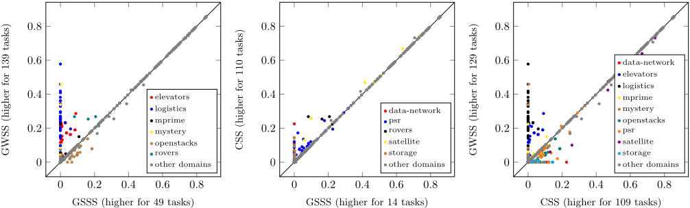
To assess the pruning power, we define the pruning ratio of a (completed) search using a pruning function as follows. We sum up, over all expanded states s, the number of all successors of s as nall and the number of generated successors of s (i.e., successors not pruned by the pruning function) as ngen. We define the pruning ratio as 1- ngen nall , yielding values from0 to 1, where 0 means that no states are pruned and 1 means that all states are pruned. Figure 2 shows scatter plots comparing the pruning ratio of all three methods, highlighting domains where the difference of the pruning ratio is above 0.1.

The results confirm the orthogonal pruning power of the methods. At the left, we compare GSSS, the previous standard in classical planning, against GWSS, the generalization introduced in this work. We observe that GWSS leads to more pruning than GSSS in 139 tasks while the converse is only true in 49 tasks. As GSSS and GWSS use the same mutexbased approximation of state-based interference and only differ in including enablers (GWSS) compared to disablers (GSSS) of applicable operators, we conclude that the former is overall more favorable in terms of pruning power. Using more sophisticated strategies for deciding when to include all disablers or all enablers could possibly increase the pruning power further. The middle plot compares GSSS against CSS. We observe that CSS, like GWSS, lead to more pruning compared to GSSS, although the differences are smaller. We learn that using state-based interference (like the mutex-based by GSSS), but including additional disablers compared to CSS, does mostly not pay off in pruning compared to the pure syntactic interference approximation used by CSS. Finally, at the right, we directly compare CSS against GWSS. We again see that GWSS are orthogonal to CSS (slightly favoring GWSS), thus also confirming our previous theoretical investigation.

We conclude that GWSS are favorable in terms of pruning compared to GSSS, and that the orthogonal pruning power of GWSS and CSS is also reflected in practice. We finally remark that the differences in pruning do not translate to large changes in coverage (i.e., number of solved tasks), which is at most 3. The technical report includes full coverage results.

7 Conclusions

We have investigated weak stubborn sets for planning in the light of the operator shifting property. We have learned that sets called weak stubborn sets in earlier work in planning are not weak stubborn sets in the original sense. Based on this finding, we have formally introduced generalized weak stubborn sets for planning, and related them to existing stubborn set approaches.

A promising direction for future research is to further relax the operator shifting property, still yielding safe pruning functions. As we have seen, the more general operator shifting property of CSS compared to stubborn sets is a result of "simply" excluding certain disabling operators. If stubborn sets are applied with syntactic interference, which is often done in practice anyway (e.g., because it allows for a more efficient implementation, see R¨oger et al., 2020), then the question arises if the operator shifting property can be further relaxed such that larger "operator blocks" are obtained, resulting in smaller sets and higher pruning power. For example, for an operator o ∈ T , can we identify cases where an operator o′ can be left out of T even though o′ is disabled by o? Can such information be synthesized algorithmically and in a generic way? Answers to such questions will potentially show ways to a further level of safe pruning functions.

Acknowledgments

We thank the anonymous reviewers for their comments, which helped improve the paper. Silvan Sievers has received funding for this work from the European Research Council (ERC) under the European Union's Horizon 2020 research and innovation programme (grant agreement no. 817639). Moreover, Silvan Sievers was partially supported by TAILOR, a project funded by the EU Horizon 2020 research and innovation programme under grant agreement no. 952215.