Learning Temporal Plan Preferences from Examples: An Empirical Study

1 Introduction

Temporal plan preferences are natural and important in a variety of applications. The PDDL3 language [Gerevini et al., 2009] provides support for their specification, and planning algorithms to handle such preferences have been deeply investigated [Edelkamp, 2006; Baier and McIlraith, 2006; Baier et al., 2009; De Giacomo et al., 2014; Torres and Baier, 2015; Camacho and McIlraith, 2019b]. Yet users often find it difficult to formalize their preferences.

In particular, our work is motivated by a recent approach to analyze dependencies between plan properties [Eifler et al., 2020a; Eifler et al., 2020b] in oversubscribed planning tasks where not all plan properties - which correspond to user preferences - can be satisfied. Rather than assuming that each preference is associated with a reward as in standard oversubscription planning [Smith, 2004; Domshlak and Mirkis, 2015], the approach analyzes which (subsets of) preferences exclude which other ones. The aim is to explicate the space of possible plans in situations where rewards are inadequate or difficult to elicit. Since the explication is done in terms of dependencies between preferences, users need to provide a sizable set of preferences spanning the aspects of plan space they are interested in. How to ease this burden?

Here we explore the possibility to learn temporal plan preferences from annotated example plans. We do so one preference at a time: our envisioned specification process is a loop over preferences to be learned, where in each iteration the user is asked to focus on one plan property of interest. We generate example plans, and the user annotates them as good/bad with respect to that property. We then leverage prior work [Neider and Gavran, 2018; Camacho and McIlraith, 2019a; Kim et al., 2019] to learn an LTL formula correctly characterizing these positive/negative examples, extracting a formalized preference. The same steps can be repeated to extract other preferences until the user stops the process.

This approach itself is fairly straightforward, and its building blocks are known. Indeed, we employ Camacho and McIlraith's [Camacho and McIlraith, 2019a] techniques, and our work is essentially an application thereof. Our contribution lies in assembling these known techniques, and empirically studying their merits for plan preference learning.

To emulate the user in systematic experiments, we employ hidden target formulas. In each preference-learning step, we:

1. fix an LTL target formula φ;
2. generate a set of example plans Π;
3. annotate each π as good (bad) if it satisfies (does not satisfy) φ; and
4. invoke LTL formula learning to extract a formula φ′ correctly characterizing these examples.

In practice, the hidden target formula φ will be inside the user's head. Emulating users in this form allows us to systematically evaluate the merits of different algorithmic methods.

We instantiate (1) with hand-made formulas suited for a collection of benchmarks, based on PDDL3 preferences as well as formula skeletons often used in model checking [Manna and Pnueli, 1990; Dwyer et al., 1999; Menghi et al., 2019]. We instantiate (4) with Camacho and McIlraith's [2019a] techniques, which learn a smallest LTL formula φ′ . The main question we consider is how to instantiate (2). TopK methods with a focus on diversity are natural candidates, as they aim at producing K good-quality (in our context: short) yet qualitatively different plans. This makes intuitive sense for our purposes as the example plans should be different, and should not be obviously bad. We experiment with three different methods from the literature [Katz et al., 2018; Katz and Sohrabi, 2020; Speck et al., 2020]. We furthermore experiment with a simple randomized version of greedy bestfirst search using hFF [Hoffmann and Nebel, 2001], which turns out to be more scalable.

We evaluate the performance of different methods as a function of domain and formula size. We investigate a variety of aspects, including not only computational effort, but also the quality of the learned formula φ′ relative to the hidden formula φ, and the quality of plan examples in the sense of how many examples are needed to learn a high-quality formula. Overall, we find that reasonable-size target formulas can often be learned effectively.

The paper is structured as follows. Section 2 gives the planning context. Section 3 describes the building blocks that we assemble in our approach, i. e., plan-generation techniques, LTL formula learning, and temporal plan preferences. Section 4 explains our system architecture and implementation. Section 5 explains the experiments setup, before we describe our empirical findings in Section 6.

2 Preliminaries

2.1 Oversubscription Planning

We are using a variant of oversubscription planning (OSP) [Smith, 2004; Domshlak and Mirkis, 2015] with finitedomain variables [B¨ackstr¨om and Nebel, 1995; Helmert, 2009]. An OSP task is a tuple τ = (V, A, c, I, Ghard , Gsoft , b). V is the set of variables, A is the set of actions, c : A→R+0 is the action cost function, and I is the initial state. Ghard (Gsoft ) is the hard (soft) goal, given as a partial assignment to V . Ghard and Gsoft are defined over disjoint sets of variables. b ∈ R+0 is the cost bound. A state is a complete assignment to V . Facts are variable-value pairs v = d. We represent partial variable assignments with sets of facts. Each action a ∈ A has a precondition prea and an effect eff a, both partial assignments to V . An action a is applicable in a state s if prea ⊆ s. Applying a to s denoted as s[[a]] results in state s′ where s′ (v) = eff a(v) for those v on which eff a is defined and s′ (v) = s(v) otherwise. The resulting state of an iteratively applicable action sequence π is denoted by s[[π]]. A plan is an action sequence π whose summed-up cost is ≤ b and where Ghard ⊆ I[[π]].

Following Eifler et al. [2020a], we do not define a plan utility over Gsoft . Instead, Gsoft is a set of temporal plan preferences (encoded into soft-goal facts [Edelkamp, 2006; Baier and McIlraith, 2006]), and the analysis they provide identifies dependencies between these (plan-space entailments, see below). The issue we tackle here is the specification of the temporal plan preferences Gsoft .

2.2 Finite Linear Temporal Logic

We use finite Linear Temporal Logic LTLf, an adaption of LTL to finite traces [Baier and McIlraith, 2006; De Giacomo and Vardi, 2013], to represent temporal preferences.

Given a planning task τ, let S be a set of symbols for all facts in τ and L(S) the set of all first-order formulas over S.

LTLf formulas are interpreted over a finite sequence of states (finite trace) σ = s0s1 · · · sn where each state si is a first-order interpretation over the symbols in S. We use the abbreviation σi for si · · · sn. Given a finite trace σ and a LTLf formula φ we say σ |= φ iff:

• σi |= final iff i = n.
• σi |= true and σi ⊭ false.
• σi |= ϕ, where ϕ ∈ L(S) iff si |= ϕ.
• σi |= ¬φ iff σi ⊭ φ.
• σi |= φ ∧ψ iff σi |= φ and σi |= ψ.
• σi |=©φ iff i < n and σi+1 |= φ
• σi |= φ U ψ iff ∃j : i ≤ j ≤ n such that σj |= ψ and ∀k : i ≤ k < j : σk |= φ

Additionally, the following standard temporal operators are used: release: φ R ψ := ¬(¬φ U ¬ψ), always: □φ := false R φ, eventually: ♦φ := true U φ, weak until: φ W ψ := (φ U ψ) ∨ □φ. The size of a LTLf formula |φ| is defined as the number of subformulas.

Part of our discussion below will draw on Eifler et al.'s [2020a] definition of plan-space entailment. Let Π be the set of plans of τ, and φ, ψ two LTLf formulas. The subset of plans that satisfy φ is denoted by MΠ(φ) := {π | π ∈ Π, π |= φ}. We write τ |= φ ⇒ ψ if MΠ(φ) ⊆ MΠ(ψ), and τ |= φ⇔ψ ifMΠ(φ) =MΠ(ψ).

3 Building Blocks

The two main building blocks of our approach are the generation of plans and the learning of LTLf formulas. In the following, we point to related work in this area, while describing the approaches we decided to use in more detail.

3.1 Plan Generation

To provide a set of sample plans Π to the user, we have to generate multiple plans for the given planning task τ. These plans ideally should cover different parts of the search space, exhibiting different possibilities to reach Ghard . Optimality with respect to plan cost is not a necessity, indeed is undesirable as it may exclude interesting plan options. So we want to allow sub-optimal plans, up to the cost bound b. Nevertheless, a bias to small plan cost can make sense as cheap plans are generally preferrable.

Given this, we explore four different plan generation techniques. Three of these are variants of top-k planning (TopK) [Katz et al., 2018; Speck et al., 2020], which is adequate as it is specifically designed to provide multiple plans. The default variant returns the best k plans in terms of cost. In domains with independent objects (like two trucks which can move independently) TopK often leads to plans which are permutations of each other. So as a second approach we use top-k planning with an additional filter, removing plans that are permutations of already found plans. This leaves us with plans that pairwise have at least one distinct action (TopKFil). Our third variant is agile diverse planning (AgDiv) by [Katz and Sohrabi, 2020] which takes not only plan quality but also solution diversity into account, and thus is a very natural approach for our purposes. It uses satisficing planning and iteratively computes new plans while forbidding all possible reorderings of already given plans.

As a simple method that actually turns out to work quite well, we also run a randomized version of hFF [Hoffmann and Nebel, 2001] in greedy best-first search (RNDhFF). The randomization adds a positive random number to each heuristic value. As this approach does not guarantee to find different plans, the plans are filtered for uniqueness in a post-process.

All of these approaches can be run as an anytime search, allowing to generate plans until a time limit is reached or a certain amount of plans is found.

3.2 Learning

There is substantial work [Neider and Gavran, 2018; Camacho and McIlraith, 2019a; Kim et al., 2019] in the area of learning LTL formulas from sample traces we can build on. The approach by [Kim et al., 2019] is based on probabilistic Bayesian models. It relies on templates so it cannot learn arbitrary LTL formulas. The probabilistic model enables robustness with respect to noise in the input data. In our context, such noise would reflect plans incorrectly annotated by the user. This could be an interesting consideration for future work, but for now we assume that such noise does not exist (the user either annotates an example plan correctly or not at all). Therefore, we follow instead other works [Neider and Gavran, 2018; Camacho and McIlraith, 2019a] that use SAT encodings to learn a smallest formula identifying the positive and negative examples perfectly. These do not rely on templates and can learn arbitrary formulas. In our implementation we use a modified re-implementation of the approach by Camacho & McIlraith [2019a].

The input of the learner are two sets of finite traces reflecting the positive and negative examples. The learning is an iterative process over the size of the learned formula. In each step a SAT encoding of all LTLf formulas with the given size and the input traces is generated. The first satisfiable assignment the SAT-solver can find is then used to reconstruct the corresponding LTLf formula. If the SAT encoding is unsatisfiable the size bound is increased.

3.3 Plan Preferences

We focus on commonly used temporal formulas in planning and model checking. We use those PDDL3 Preferences [Gerevini et al., 2009] that do not have a numeric argument. Additionally, we include templates often used in model checking [Manna and Pnueli, 1990; Dwyer et al., 1999; Menghi et al., 2019]. Table 1 lists the formula templates we will consider (for the construction of hidden target formulas) in our empirical evaluation. While these do not exploit the full expressiveness of LTLf, arguably user preferences tend to be temporally simple (reflected for example in the fact that PDDL3 caters for only a small fraction of LTLf.

4 Architecture

We now discuss how to assemble these building blocks into an architecture for plan preference learning. We first briefly re-explain the workflow in our approach, highlighting the issues and relevant special cases that can arise. We then briefly outline our implementation. Recall in what follows that in our experiments we will assume a hidden target formula, denoted φt, inside the user's head.

4.1 Workflow: Issues and Special Cases

Step 1: Plan Generation. In the first step we generate a set Πg of plans for the given planning task, using one of the introduced approaches RNDhFF, TopK, TopKFil or AgDiv. As φt is hidden, the plan generation cannot be tailored to generate positive and negative examples for φt. So we simply consider the first n plans generated. We will experimentally explore the impact of the parameter n.

An important complication is that the learning step requires at least one example from each class, i. e., at least one positive and at least one negative example. Obviously this may not be true in the first n plans, in which case one has to either give up or increase the value of n. An issue with the latter is that the hidden user preference may actually be a tautology in the planning task, i. e., may be true (or false) in all plans. In practice we won't be able to check that. Note though that tautological preferences are not meaningful (they do not distinguish between plans at all). Presumably, users will typically know enough about the task at hand to come up with meaningful preferences only. In our experiments, we consider only non-tautological preferences.

Step 2: Plan Annotation. We provide the set of plans Πg to the user and ask her to annotate the plans with respect to her hidden target preference φt as positive Πp and negative Πn examples. Clearly, the number n of plans the user has to annotate should be as small as possible. We will evaluate empirically how many plans are necessary to learn φt.

Importantly, in practice, one could interleave plan annotation and formula learning until the user is satisfied with the result. In our setting here, this corresponds to analyzing learning performance as a function of n.

Step 3: Learning. Given Πp and Πn, we call the learner to obtain the set Φl of smallest LTLf formulas perfectly identifying Πp and Πn. As φt is not known, Φl can not be filtered further without additional information from the user. Hence all formulas in Φl are forwarded to the user for inspection.

Observe that the formulas φl ∈ Φl can be related to the target formula φt in exactly one of the following ways:

• (a) we learn the same formula: φl = φt
• (b) φl is equivalent to φt: τ |= φl ⇔φt
• (c) φl is an overapproximation of φt: τ |= φl ⇒φt
• (d) φl is an underapproximation of φt: τ |= φt ⇒φl
• (e) no direct relation, i. e., none of (1)-(4) holds.

Case (a) is the ideal case and provides the result the user is expecting. In the worst case (e), the user is confronted with a set of formulas not related to what she has in mind at all.

The intermediate cases are more difficult to judge. As for equivalence (b), this may seem unproblematic, but depending on how similar φl and φt are, the user may not be able to recognize the equivalence. In our experiments, we observed surprising equivalent formulas, that identified subtle dependencies in the planning task. On the positive side though, this form of dependency identification constitutes an alternative application of our techniques, as a new form of plan-space explication in the sense of Eifler et al. [2020a]. The plan annotation and formula learning then used to automatically find new formulas that relate in particular ways to previously identified preferences. We illustrate this possible alternative use of our techniques at the end of the experiments (Section 6.5).

The usefulness of over/under-approximations (c) and (d) of φt also highly depends on their similarity to φt. A useful result would for example be φl = □a given the target formula φt = □(a ∨ b), or in general if φl → φt based on the LTLf semantic regardless of the planning task. In our experiments we often observed that the learning identified instead subtle unexpected dependencies, again suggesting the abovementioned alternative use in the sense of Eifler et al. [2020a].

4.2 Implementation

For plan generation we used the publicly available implementations of SymK [Speck et al., 2020] for TopK and TopKFil, forbiditerative [Katz and Sohrabi, 2020] for AgDiv, and Fast Downward [Helmert, 2006] for RNDhFF. The plan selection for TopKFil is supported by SymK as an internal filter. We extended the translator of each planner by the LTLf compilation implementation by [Eifler et al., 2020b]. This is required for our experimental setup as explained in the next section.

The preferences we consider are LTLf formulas over facts. To convert plans to lists of fact sets we use VAL [Howey et al., 2004]. We discard the static facts (that are always true, e. g. defining the road connections in transportation domains).

The implementation we use for LTLf learning is a reimplementation of Camacho & McIlraith's tool [Camacho and McIlraith, 2019a]. The original implementation only outputs one formula of the given size. As we do not have a reason to prefer one formula over another, we extended the implementation to provide all formulas of that size: we call the SAT solver repeatedly, adding a new clause each time to enforce that previously found formulas are excluded.

5 Experiment Setup

Some words are in order regarding our benchmark design and other particularities of our experiments setup.

5.1 Benchmark Design

The planning instances we consider are based on the resource-constrained planning instances used by Eifler et al. [Eifler et al., 2020a]. These consist of variants of Blocksworld, Nomystery, Rovers and TPP. In all domains, the action-cost budget b is set to 1.5 times the optimal cost necessary to achieve all hard goals (this setting allows to achieve some, but not very many, additional temporal soft goals). The Blocksworld is a version with two hands. Nomystery is a simple transportation domain over a road-map graph. In TPP, multiple markets offer different goods, which need to be bought and transported to a depot. In Rovers, one has to navigate a road map, take rock/soil samples, and take pictures of objectives with limited view. From each of these domains we selected 10 instances with a fixed number of hard goals (Blocksworld 6, Nomystery 4, Rovers 6 and TPP 4).

To generate hidden target formulas for our experiments, we used the LTL templates given in Table 1. For each planning task τ = (V,A, c, I,Ghard ,Gsoft , b) we iteratively instantiated each template with random facts from ⋃a∈A eff a. For templates up to size 4 we also included extended versions, by instantiating a or b with a conjunction or disjunction of two facts. Then, for each candidate formula φ we checked whether φ is non-tautological: (τ, φ) is added to our benchmark set only if both Ghard ∪ {φ} and Ghard ∪ {¬φ} are solvable. For each task τ , we included at most two formulas based on the same template. To guaranty termination we skip a template after at most 30 failed candidate formula checks. This procedure generated on average 30 formulas per task, resulting in a benchmark set of 1284 task-formula pairs.

5.2 Hypothetical Best-Case for Plan Generation

In practice, plan generation cannot be tailored to the planning formula φt, as that is hidden in the user's head. Yet, intuitively, it is important for the example plans to be balanced: same numbers of positive and negative instances. A highly imbalanced set of examples can be expected to impede formula learning, as it will fail to clarify the distinction line between the two classes.

We evaluate this hypothesis here by exploring two different setups for plan generation: the realistic application setup Genapp where plans are generated without knowledge of φt; vs. the hypothetical idealized setup Genideal where we generate perfectly balanced example plan sets by enforcing φt and ¬φt each in half of the plan-generation runs. (Kim et al.'s [2019] experiment setup featured a related construction.)

The idealized setup also serves to shed light on what could potentially be achieved in future work by advanced methods trying to incorporate partial information about the user preference (i. e., what kinds of structures are of interest).

5.3 Evaluation with Respect to the Target Formula

In our experiments, to evaluate the quality of the learned formula, our foremost criterion naturally is the degree of direct relation to the hidden target formula φt, according to the categories (a)-(e) discussed in Section 4.1. Note that checking these relations involves expensive implication tests, identifying entailments in plan space. Our implementation works as follows. The context of each test is a planning task τ with hard goals Ghard . Given target formula φt and learned formula φl, we test whether (1) τ |= φl ⇒ φt and (2) τ |= φt ⇒ φl. Each of these tests is performed through compilation into a modified planning task, namely Ghard ∪ {φl, ¬φt} for (1) and Ghard ∪ {¬φl, φt} for (2), where LTL hard goals are encoded through compilation into goal facts. Each test succeeds iff the corresponding planning task is unsolvable.

All experiments were run on Intel E5-2660 machines running at 2.20 GHz with a memory limit of 4GB. The example plan generation and the formula learning had time limits of 30min each. As evaluating φt with respect to φl can be very time consuming, we used a timeout of 2h for this step. For Genapp we generated up to 50 example plans, and for Genideal we generated up to 25 positive and 25 negative examples.

6 Experimental Results

Our evaluation is structured into five parts. The first two parts evaluate plan generation, in terms of computational performance, and the balance of the resulting plan sets. The third part evaluates the quality of the learned formulas relative to the hidden target formula, as a function of target formula size, plan generation method, and number n of annotated example plans. In the fourth part we give some illustrative examples and conclude in the fifth part with a brief evaluation of the alternative application of our techniques as a new form of planspace explication.

6.1 Plan Generation: Computational Performance

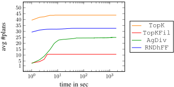
Figure 1 shows the average number of plans generated over time. Top-k planning (TopK) clearly produces most plans fastest, followed by randomized hFF (RNDhFF). Agile diverse planning (AgDiv) generates about half of the requested 50 plans within the given time limit. Top-k planning with permutation filter (TopKFil) is least apt at generating many example plans; the permutation filtering turns out to be quite aggressive given the top-k search output, effectively cutting off plan generation after a few seconds.

6.2 Plan Generation: Balance

At least one positive and negative example is necessary for the learning step. So the first question is in how many of our 1284 benchmark instances (task-formula pairs) this is the case. The answer is: 205 for TopK, 536 for TopKFil, 659 for AgDiv, and 628 for RNDhFF. The most striking observation concerns TopK, which generates the largest number of example plans, yet often yields examples of only one category. This is due to its tendency to generate plan permutations.

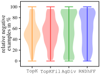
In what follows, we consider, for each plan-generation method, only those benchmark instances where both positive and negative example plans are generated. The set of all these benchmark instances (union across plan-generation methods) is denoted Ip&n. Figure 2 (left) evaluates how balanced the sets of example plans are for each plan-generation method.

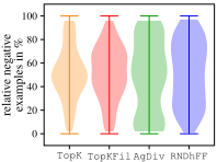
It may seem surprising here at first, given the above, that TopK generates the most balanced example plan sets within Ip&n. On closer inspection, this is somewhat due to the smaller benchmark basis underlying the data for TopK. As Figure 2 (right) shows, on these 205 benchmark instances also AgDiv and RNDhFF tend to be more balanced. Overall, the superior plan generation algorithm in terms of balancedness is TopKFil, which exhibits strong behavior especially for target formulas relating to reachability (e.g. ♦φ).

6.3 Quality of Learned Formulas

Figure 3 provides our evaluation of learning quality. Our main criterion for assessing quality are categories (a)-(e) relative to the target formula. We say that an instance is solved if either the target formula or an equivalent formula is learned.

Consider first the leftmost part of the figure. It provides data for the realistic plan-generation setup Genapp where the hidden target formula is not taken into account in plan generation. To make the complete picture visible, we also include those cases where learning was not possible as only positive/negative example plans were generated. For very small formulas (size 2 and 3), all plan generation approaches solve a large fraction of those benchmark instances (Ip&n) where learning could be run. For larger target formulas performance drops sharply though, with less than a quarter of the benchmark instances being solved.

Comparing across plan-generation methods, up to size 5, AgDiv is best, closely followed by RNDhFF and TopKFil. For larger sizes, there is no superior method. This ranking of plan generation approaches is exactly the ranking according to the number of instances in Ip&n (659 AgDiv, 628 RNDhFF, 536 TopKFil, 205 TopK). While TopK tends to produce highly balanced plan sets (Figure 2), it does not produce a notably better ratio of high-quality learned formulas.

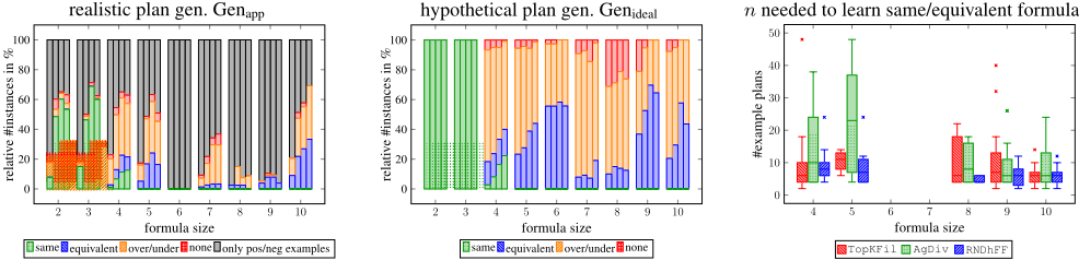
Turning now to the middle part of Figure 3, we vividly see that the bottleneck of our approach is the quality of plan generation. Recall that in Genideal, the plan-generation methods have access to the target formula and produce perfectly balanced example plan sets. Learned-formula quality increases dramatically relative to Genapp, with formula sizes 1 and 2 consistently solved perfectly, equivalent formulas learned frequently even for large formulas, and formulas unrelated to the target learned almost never. The key question for future work is how to alleviate this performance gap between Genapp and Genideal. We get back to this in the conclusion.

Consider finally the rightmost part of Figure 3, which provides an evaluation of plan-generation methods in terms of the number n of example plans needed to solve a benchmark instance. To enable a meaningful comparison, we require commonly solved benchmarks, need to exclude TopK, and exclude uninteresting instances solved by any method with n = 1. Given these restrictions, Genapp does not provide a sufficient basis for a meaningful comparison, so we consider Genideal instead. Overall RNDhFF performs best. Its median is never larger than n = 10, and variance is small. TopKFil and AgDiv in contrast frequently suffer from high n. We emphasize that these results are important, as annotating many example plans (larger n) is a burden on the user.

6.4 Illustration: Example Learned Formulas

Let's consider some examples for illustration, covering the different possible relations to the target formula.

For simple ordering constraints like the Rovers target formula ¬have-soil-analysis(r0,w0) U at(r1,w2), often the exact target formula is learned. For the target formula ♦(in(p1, t1)∨at(t1, l5)) in Nomystery, we learned the smaller equivalent formula ♦in(p1, t1), which is obviously an underapproximation though equivalence is difficult to see. In TPP, the underapproximation ♦at(t1,m0) learned for the target ¬at(t0,m0) U at(t1,m0) should also be recognizable.

One bad case is the target formula □¬(holding(b2, h0) ∨ holding(b0, h1)), restricting the hand usage for two blocks in Blocksworld. On this benchmark instance, we learned the overapproximation ¬holding(b2, h0) U holding(b0, h0). Although the formulas partially contain the same facts, it is quite difficult to determine how they relate to each other.

6.5 Alternative Use: Plan Space Explication

While learned formulas not identical to the target formula may not be easily recognizable to the user, as mentioned before they can also serve for plan space explication in the sense of Eifler et al. [2020a]. In this alternative application setting, the task is not to learn a hidden target formula, but instead to automatically identify new formulas entailing, or entailed by, a known (previously already specified) plan preference φt. This may elucidate non-obvious properties of plan space.

For illustration, in TPP for target formula ♦at(t1,m1) we learn the underapproximation ♦¬at(t1, d), and hence uncover the entailment τ |= ♦¬at(t1, d) ⇒ ♦at(t1,m1) which shows that, if truck t1 leaves depot d, then it must visit market m1. In Blocksworld for target formula ♦(ontable(b4)∧ontable(b1)) we learn the overapproximation clear(b3) U ontable(b1), and uncover the entailment τ ′ |= ♦(ontable(b4) ∧ ontable(b1)) ⇒ clear(b3) U ontable(b1) which shows that, if b1 and b4 are both on the table at some point, then b3 must stay clear until b1 is on the table.

7 Conclusion

We have assembled technology learning user preferences from annotated plan examples. The results are encouraging and constitute a first step towards the deeper investigation of this form of preference elicitation in planning.

The key question for future work is how to alleviate the large performance gap between practical plan generation (without access to the hidden target formula) and idealized plan generation (with such access). Presumably, addressing this requires some information about the target formula, e. g. what kinds of objects or predicates are of interest, which formula templates/temporal structures are of interest, etc. Given such information, it may be possible to devise plan-diversity measures tailored to produce balanced example sets.

Acknowledgments

This material is based upon work supported by the Air Force Office of Scientific Research under award number FA955018-1-0245, and by the German Research Foundation (DFG) under grant 389792660 as part of TRR 248 (see https:// perspicuous-computing.science).