
Anytime Multi-Agent Path Finding via Large Neighborhood Search
Proceedings of the Thirtieth International Joint Conference on Artificial Intelligence. Main Track. Pages 4127-4135.
https://doi.org/10.24963/ijcai.2021/568
Keywords
- Agent-based and Multi-agent Systems: Multi-agent Planning
- Planning and Scheduling: Search in Planning and Scheduling
- Robotics: Motion and Path Planning
Abstract
Multi-Agent Path Finding (MAPF) is the challenging problem of computing collision-free paths for multiple agents. Algorithms for solving MAPF can be categorized on a spectrum. At one end are (bounded-sub)optimal algorithms that can find high-quality solutions for small problems. At the other end are unbounded-suboptimal algorithms that can solve large problems but usually find low-quality solutions. In this paper, we consider a third approach that combines the best of both worlds: anytime algorithms that quickly find an initial solution using efficient MAPF algorithms from the literature, even for large problems, and that subsequently improve the solution quality to near-optimal as time progresses by replanning subgroups of agents using Large Neighborhood Search. We compare our algorithm MAPF-LNS against a range of existing work and report significant gains in scalability, runtime to the initial solution, and speed of improving the solution.
- [Barer et al., 2014] Max Barer, Guni Sharon, Roni Stern, and Ariel Felner. Suboptimal variants of the conflict-based search algo- rithm for the multi-agent pathfinding problem. In SoCS, pages 19-27, 2014.
- [Björdal et al., 2020] Gustav Björdal, Pierre Flener, Justin Pearson, Peter J. Stuckey, and Guido Tack. Solving satisfaction problems using large-neighbourhood search. In CP, pages 55-71, 2020.
- [Boyarski et al., 2015a] Eli Boyarski, Ariel Felner, Guni Sharon, and Roni Stern. Don't split, try to work it out: Bypassing con- flicts in multi-agent pathfinding. In ICAPS, pages 47-51, 2015.
- [Boyarski et al., 2015b] Eli Boyarski, Ariel Felner, Roni Stern, Guni Sharon, David Tolpin, Oded Betzalel, and Solomon Eyal Shimony. ICBS: Improved conflict-based search algorithm for multi-agent pathfinding. In IJCAI, pages 740-746, 2015. IJCAI
- [Boyarski et al., 2020] Eli Boyarski, Ariel Felner, Daniel Harabor, Peter J. Stuckey, Liron Cohen, Jiaoyang Li, and Sven Koenig. Iterative-deepening conflict-based search. In IJCAI, pages 4084- 4090, 2020. IJCAI
- [Cohen et al., 2018] Liron Cohen, Matias Greco, Hang Ma, Carlos Hernández, Ariel Felner, T. K. Satish Kumar, and Sven Koenig. Anytime focal search with applications. In IJCAI, pages 1434- 1441, 2018. IJCAI
- [Demir et al., 2012] Emrah Demir, Tolga Bektas, and Gilbert La- porte. An adaptive large neighborhood search heuristic for the pollution-routing problem. European Journal of Operational Re- search, 223(2):346-359, 2012.
- [Erdmann and Lozano-Perez, 1987] Michael Erdmann and Tomas Lozano-Perez. On multiple moving objects. Algorithmica, 2(1- 4):477, 1987.
- [Gange et al., 2019] Graeme Gange, Daniel Harabor, and Peter J. Stuckey. Lazy CBS: Implicit conflict-based search using lazy clause generation. In ICAPS, pages 155-162, 2019.
- [Goldberg, 1989] David E. Goldberg. Genetic Algorithms in Search Optimization and Machine Learning. Addison-Wesley, 1989.
- [Hoang et al., 2018] Khoi D. Hoang, Ferdinando Fioretto, William Yeoh, Enrico Pontelli, and Roie Zivan. A large neighboring search schema for multi-agent optimization. In CP, pages 688- 706, 2018.
- [Lam and Bodic, 2020] Edward Lam and Pierre Le Bodic. New valid inequalities in branch-and-cut-and-price for multi-agent path finding. In ICAPS, pages 184-192, 2020.
- [Laurent et al., 2021] Florian Laurent, Manuel Schneider, Chris- tian Scheller, Jeremy D. Watson, Jiaoyang Li, Zhe Chen, Yi Zheng, Shao-Hung Chan, Konstantin Makhnev, Oleg Svid- chenko, Vladimir Egorov, Dmitry Ivanov, Aleksei Shpilman, Ev- genija Spirovska, Oliver Tanevski, Aleksandar Nikov, Ramon Grunder, David Galevski, Jakov Mitrovski, Guillaume Sartoretti, Zhiyao Luo, Mehul Damani, Nilabha Bhattacharya, Shivam Agarwal, Adrian Egli, Erik Nygren, and Sharada P. Mohanty. Flatland competition 2020: MAPF and MARL for efficient train coordination on a grid world. In PMLR, 2021.
- [Li et al., 2019a] Jiaoyang Li, Ariel Felner, Eli Boyarski, Hang Ma, and Sven Koenig. Improved heuristics for multi-agent path find- ing with conflict-based search. In IJCAI, pages 442-449, 2019. IJCAI
- [Li et al., 2019b] Jiaoyang Li, Daniel Harabor, Peter J. Stuckey, Hang Ma, and Sven Koenig. Symmetry-breaking constraints for grid-based multi-agent path finding. In AAAI, pages 6087-6095, 2019.
- [Li et al., 2020] Jiaoyang Li, Graeme Gange, Daniel Harabor, Pe- ter J. Stuckey, Hang Ma, and Sven Koenig. New techniques for pairwise symmetry breaking in multi-agent path finding. In ICAPS, pages 193-201, 2020.
- [Li et al., 2021a] Jiaoyang Li, Zhe Chen, Daniel Harabor, Peter J. Stuckey, and Sven Koenig. Anytime multi-agent path finding via large neighborhood search: Extended abstract. In AAMAS, pages 1581-1583, 2021.
- [Li et al., 2021b] Jiaoyang Li, Zhe Chen, Yi Zheng, Shao-Hung Chan, Daniel Harabor, Peter J. Stuckey, Hang Ma, and Sven Koenig. Scalable rail planning and replanning: Winning the 2020 flatland challenge. In ICAPS, pages 477-485, 2021.
- [Li et al., 2021c] Jiaoyang Li, Wheeler Ruml, and Sven Koenig. EECBS: Bounded-suboptimal search for multi-agent path find- ing. In AAAI, pages 12353-12362, 2021.
- [Ropke and Pisinger, 2006] Stefan Ropke and David Pisinger. An adaptive large neighborhood search heuristic for the pickup and delivery problem with time windows. Transportation Science, 40(4):455-472, 2006.
- [Sajid et al., 2012] Qandeel Sajid, Ryan Luna, and Kostas E. Bekris. Multi-agent pathfinding with simultaneous execution of single-agent primitives. In SoCS, pages 88-96, 2012.
- [Sharon et al., 2015] Guni Sharon, Roni Stern, Ariel Felner, and Nathan R. Sturtevant. Conflict-based search for optimal multi- agent pathfinding. Artificial Intelligence, 219:40-66, 2015.
- [Shaw, 1998] Paul Shaw. Using constraint programming and local search methods to solve vehicle routing problems. In CP, pages 417-431, 1998.
- [Song et al., 2020] Jialin Song, Ravi Lanka, Yisong Yue, and Bis- tra Dilkina. A general large neighborhood search framework for solving integer programs. In NeurIPS, 2020.
- [Standley and Korf, 2011] Trevor Scott Standley and Richard E. Korf. Complete algorithms for cooperative pathfinding problems. In IJCAI, pages 668-673, 2011. IJCAI
- [Stern et al., 2019] Roni Stern, Nathan R. Sturtevant, Ariel Felner, Sven Koenig, Hang Ma, Thayne Walker, Jiaoyang Li, Dor Atz- mon, Liron Cohen, T. K. Satish Kumar, Eli Boyarski, and Ro- man Bartak. Multi-agent pathfinding: Definitions, variants, and benchmarks. In SoCS, pages 151-159, 2019.
- [Vedder and Biswas, 2021] Kyle Vedder and Joydeep Biswas. X*: Anytime multi-agent path finding for sparse domains us- ing window-based iterative repairs. Artificial Intelligence, 291:103417, 2021.
- [Wang and Botea, 2011] Ko-Hsin Cindy Wang and Adi Botea. MAPP: a scalable multi-agent path planning algorithm with tractability and completeness guarantees. Journal of Artificial Intelligence Research, 42:55-90, 2011.
- [Wang and Goh, 2015] Wenjie Wang and Wooi Boon Goh. An it- erative approach for makespan-minimized multi-agent path plan- ning in discrete space. Autonomous Agents and Multi-Agent Sys- tems, 29(3):335-363, 2015.
- [Yu and LaValle, 2013] Jingjin Yu and Steven M. LaValle. Struc- ture and intractability of optimal multi-robot path planning on graphs. In AAAI, pages 1444-1449, 2013.
References were extracted automatically from the PDF and may contain errors.
Full text extracted automatically from the PDF; figures, tables and equations may differ. The PDF is the version of record.
1 Introduction
Multi-Agent Path Finding (MAPF) asks us to plan collisionfree paths for a team of moving agents: each from a start location to a target location. MAPF is important for a wide variety of application areas, including computer games, robotics, and traffic management. For such applications, MAPF instances can involve hundreds and sometimes thousands of agents. Desirable solutions are those which can be computed quickly but which also minimize an operational objective, such as the sum of costs or makespan. Unfortunately, MAPF is NP-hard to solve optimally [Yu and LaValle, 2013].
One category of leading MAPF algorithms is optimal and bounded-suboptimal algorithms, which guarantee to return a solution that is not larger than optimal by more than some fixed multiplicative factor. The main drawback is their scalability: problems with hundreds of agents are considered extremely challenging, and timeout failures are common. Another category of leading MAPF algorithms is unboundedsuboptimal algorithms, which trade optimality guarantees for speed and which can scale to thousands of agents. Here, planning is very fast because coordination is achieved by using pre-determined movement rules or by planning the agents one after the other in some specified order. The main drawback is their solution quality: the computed solution can be far from optimal, which is usually undesirable for applications.
In this work, we consider an alternative and anytime approach to solving MAPF. First, we aim to find an initial solution fast so that one is usually available, even for extremely challenging problems. We experiment with a variety of MAPF algorithms from the existing literature. Next, if more time is available, we aim to reduce the cost of the incumbent solution by replanning subgroups of agents. We employ Large Neighborhood Search (LNS) [Shaw, 1998], a well-known meta-heuristic framework from combinatorial optimization. We propose a variety of destroy heuristics and repair operators specific to MAPF. Each destroy heuristic selects a subset of agents and discards their current paths. Each repair operator finds new paths for the selected agents with the objective of reducing their overall cost.
We evaluate our algorithm MAPF-LNS in an extensive set of experiments and report large gains over a variety of competing algorithms from the recent literature, including oneshot bounded- and unbounded-suboptimal algorithms and other anytime algorithms. In contrast to the existing work, MAPF-LNS can be understood as a near-optimal algorithm (with no guarantee), which combines the strengths of leading algorithms from across the algorithmic spectrum in the sense that we (i) compute initial solutions fast; (ii) find near-optimal solutions eventually; and (iii) scale to very large numbers of agents. This paper is an extension of [Li et al., 2021a].
2 MAPF Definition
MAPF is a broad family of problems with many variants [Stern et al., 2019]. In this paper, we use a common formulation that considers: (i) vertex and swapping conflicts, (ii) the "stay at target" assumption, and (iii) the objective of minimizing the sum of (individual path) costs. Nevertheless, the proposed algorithm MAPF-LNS is flexible and can be easily adapted to other MAPF formulations.
Formally, MAPF takes as input a graph G = (V,E) and a set of m agents A = {a1, . . . , am}. Each agent ai ∈ A has a start vertex si ∈ V and a target vertex gi ∈ V . At each discretized timestep, an agent can either move to an adjacent vertex or wait at its current vertex. A path pi for agent ai is a sequence of vertices which are adjacent (i.e.,
(pi[t], pi[t + 1]) ∈ E, indicating a move action) or identical (i.e., pi[t] = pi[t + 1], indicating a wait action) and which starts at si and ends at gi. We assume that the agents remain at their goal vertices forever after completing their paths. The length l(pi) of path pi is the number of its constituent edges (i.e., move and wait actions). The distance d(x, y) from vertex x to vertex y is the length of the shortest path from x to y. The delay delay(pi) = l(pi) - d(si, gi) of path pi is the difference between its length and the distance between its endpoints si and gi. A collision occurs when two agents attempt to occupy the same vertex or traverse the same edge in opposite directions at the same timestep. A solution is a set of collision-free paths, one for each agent. Our task is to find a solution P = {pi | ai ∈ A} that minimizes its sum of costs ∑ai∈A l(pi), which is equivalent to minimizing its sum of delays ∑ai∈A delay(pi).
3 ExistingMAPF Algorithms
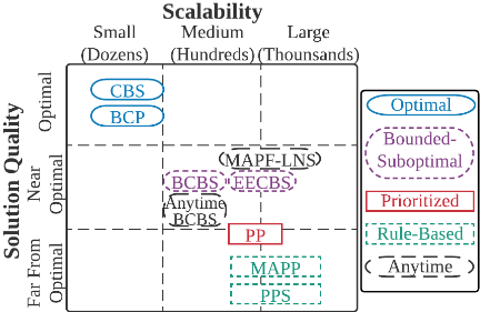
We categorize the existing algorithms below and provide a rough comparison of them in Figure 1, together with an entry for our new algorithm MAPF-LNS.
Optimal algorithms include A*-based algorithms and compilation-based algorithms. The leading algorithms in this category often deploy a strategy of planning paths for each agent independently by ignoring other agents first and resolving collisions afterward, such as CBS [Sharon et al., 2015; Gange et al., 2019; Li et al., 2020] and BCP [Lam and Bodic, 2020]. However, due to their time complexity, they can find optimal solutions only for small or medium-sized instances and run out of time or memory for other instances.
Bounded-suboptimal algorithms are usually variants of optimal algorithms, such as the CBS variants BCBS [Barer et al., 2014] and EECBS [Li et al., 2021c]. They scale to larger instances than optimal algorithms but still provide guarantees on the solution quality. However, they are still exponentialtime algorithms and thus also have limited scalability. Even if a large suboptimality bound is used, they can still run out of time or memory when solving hard instances.
Prioritized algorithms plan paths based on a priority ordering of the agents. For example, Prioritized Planning (PP) [Erdmann and Lozano-Perez, 1987] plans a shortest path for each agent one after the other in the order from high to low-priority agents that avoids collisions with the (already planned) paths of higher-priority agents. Although prioritized algorithms can scale to large instances, they do not provide guarantees on completeness or solution quality.
Rule-based algorithms, such as MAPP [Wang and Botea, 2011] and Parallel-Push-and-Swap (PPS) [Sajid et al., 2012], plan paths via simple movement rules. Although many of them guarantee to find solutions in polynomial time and can solve extremely congested instances (with a high ratio of the number of agents over the number of vertices in the graph), their solution quality has no guarantees and is always substantially worse than that of other algorithms.
The algorithms described above have different aims and tradeoffs in terms of suboptimality, scalability, and completeness. Interestingly, anytime behavior, i.e., generating an initial solution fast and improving it over time, is not the focus of them. In practice, anytime behavior is highly desirable: (bounded-sub)optimal algorithms that fail to find a solution for the large-sized instances encountered in applications are not acceptable, while unbounded-suboptimal algorithms are not attractive if their solution is far from optimal. There is little existing work on anytime algorithms: OA [Standley and Korf, 2011] and X* [Vedder and Biswas, 2021] achieves the anytime behavior by repeatedly calling A* to find optimal solutions for larger and larger sub-problems and are effective only for non-congested instances. IMMI [Wang and Goh, 2015] repeatedly replan single-agent paths to reduce the makespan (instead of the sum of costs) of the solution over time. The optimal algorithm BCP [Lam and Bodic, 2020] uses a branch-and-bound algorithm, which is anytime in theory, but rarely finds solutions much earlier than the optimal in practice [Li et al., 2021c]. Anytime BCBS [Cohen et al., 2018] adapts the high-level focal search of the bounded-suboptimal algorithm BCBS [Barer et al., 2014] to anytime focal search. It starts with an infinite bound on the sum of costs objective, which is then repeatedly tightened to S - 1 whenever a new solution with the sum of costs S is found.
4 Large Neighborhood Search for MAPF
Large Neighborhood Search (LNS) [Shaw, 1998] is a popular meta-heuristic for finding good solutions to challenging discrete optimization problems. Starting from a given solution, we delete part of the solution, called a neighborhood, and treat the remaining part of the solution as fixed. What results is a simpler form of the original problem to solve. We can use whatever approach we desire to solve the reduced problem, assuming that it can take into account the fixed information. If the new solution found is better than the current solution, we replace the current solution with the new solution.
Although LNS is widely used for solving different optimization problems [Hoang et al., 2018; Bj¨ordal et al., 2020; Song et al., 2020], we are unaware of any previous LNS approaches for MAPF. Given a MAPF instance, we first call a MAPF algorithm to find an initial solution P. Any nonoptimal algorithms can be used here. Then, in each iteration, we select a subset of agents As ∈ A, remove their paths P - s = {pi ∈ P | ai ∈ As} from P, and replan new paths
Input: Graph G = (V, E), agents A = {a1, . . . , am}, neighborhood size N, paths of the agents P = {p1, . . . , pm}, and tabu list tabuList 1 ak ← argmaxai∈A\tabuList {delay(pi)}; 2 tabuList ← tabuList ∪ {ak}; 3 if |tabuList| =m∨ delay(pk) = 0 then 4 tabuList ← ∅; 5 As ← {ak}; 6 while |As| < N do 7 As ← RANDOMWALK(G, ak, P,As,N); 8 ak ← a random agent in As; 9 return As; 10 Function RANDOMWALK(G, ak, P,As,N) : 11 (x, t) ← (pk[t], t), where t is a random timestep in [0, l(pk)); 12 Nx ← {v ∈ V | (x, v) ∈ E ∪ {(x, x)} ∧ t + 1 + d(v, gk) < l(pk)}; 13 while |Nx| > 0 ∧ |As| < N do 14 y ← a random vertex in Nx; 15 As ← As ∪ {ai ∈ A | pi[t + 1] = y ∨ (pi[t] = y ∧ pi[t + 1] = x)}; 16 (x, t) ← (y, t + 1); 17 Nx ← {v ∈ V | (x, v) ∈ E ∪ {(x, x)} ∧ t + 1 + d(v, gk) < l(pk)}; 18 return As;for them by calling a modified MAPF algorithm. The modified algorithm returns a set of paths P + s , one for each agent in As, that do not collide with each other and with the paths in P. Most optimal, bounded-suboptimal, and prioritized algorithms can be adapted to this modified variant by treating the paths in P as moving obstacles. We then compare the (old) path set P - s with the (new) path set P + s and add the one with the smaller sum of costs to P. We repeat this procedure until we time out. We call the resulting algorithmMAPF-LNS.
5 Neighborhood Selection
The selection of good neighborhoods for exploration is critical to the success of LNS. For adaptive LNS (introduced in the next section) to be most successful, the neighborhoods should be orthogonal, in the sense that they are formed very differently. Therefore, in this section, we define three different neighborhood-selection heuristics for MAPF. We use a predefined parameter N to specify the number of agents that we want to put in one neighborhood.
5.1 Agent-Based Neighborhood
The first heuristic is based on the agents and their paths. We want to select an agent whose path could be shorter if some other agents were not blocking its way, as replanning them together has a chance to reduce the overall costs of their paths.
Algorithm 1 shows the pseudo-code. We first choose the agent ak that is not in the tabu list (i.e., a globally maintained set, initially being empty, to avoid selecting the same agent repeatedly) and whose path has the largest delay [Line 1]. We update the tabu list by adding agent ak to it [Line 2]. In case that the agents being delayed are all in the tabu list or the path of agent ak has a delay of zero (indicating that the path of any agent that is not in in the tabu list has a delay of zero), we empty the tabu list [Lines 3 and 4]. We then initialize the neighborhood As with agent ak [Line 5] and let the agent perform a restricted random walk (with details introduced in the next paragraph) to collect the agents that prevent it from reaching its target vertex gk earlier. These agents are added to the neighborhood As as well [Line 7]. We randomly select an agent in As [Line 8], which could be the same agent or a different agent, and repeat the procedure as long as fewer than N agents are in As [Line 6]. In the experiments, we iterate for at most 10 iterations (not shown in the pseudo-code) to address the situation where the agent density is too low for us to collect N agents in As.
In function RANDOMWALK(G, ak, P,As,N), agent ak performs a restricted random walk, which allows it to take only the move or wait actions that could potentially lead to a path shorter than its current one, ignoring collisions with the paths in P. Then, the agents that agent ak collides with during the random walk are the ones that might prevent agent ak from reaching its target vertex gk earlier and thus added to As. Formally, we first randomly choose a start state (i.e., a vertextime pair) along the path of agent ak for the random walk, i.e., a vertex x along path pk at some timestep t ∈ [0, l(pk)) [Line 11]. We then collect the possible vertices Nx of agent ak at timestep t + 1 that might be on shorter paths to gk (ignoring other agents) than its current path pk [Line 12]. More specifically, d(v, gk) is the length of a shortest path from vertex v to vertex gk (ignoring other agents). So, the length of a path for agent ak that visits vertex v at timestep t+1 is at least t+1+d(v, gk). Thus, if t+1+d(v, gk) < l(pk), then agent ak might be able to reach gk via vertex v at timestep t + 1 earlier than by following path pk. As long as the vertex set Nx is not empty and we have not yet collected enough agents in As [Line 13], we let the agent move to a random vertex y in Nx [Line 14] and add any agents to As whose paths collide with this action [Line 15]. Lastly, we update the state of agent ak [Line 16] and the vertex set Nx [Line 17].
5.2 Map-Based Neighborhood
The second heuristic is based on the topology of the map (= graph). In particular, we are interested in the agents that visit the same intersection vertex, i.e., a vertex with a degree greater than 2, because a different ordering of the agents to traverse an intersection vertex could lead to solutions of different qualities. In case that there are not enough agents at one intersection vertex, we explore the map around the intersection vertex to find nearby intersection vertices and collect agents that visit them as well. This neighborhood is orthogonal by design from the agent-based neighborhood.
Algorithm 2 shows the pseudo-code. We begin by collecting all intersection vertices [Line 1] and picking a random one [Line 2]. We put this vertex into a queue [Line 3] and perform a breadth-first search from it. Every time when we pop a vertex x from the queue [Line 6], we examine whether it is an intersection vertex [Line 7]. If it is, we add the agents that visit vertex x to the neighborhood As [Line 8] (with details introduced in the next paragraph). We then add the vertices
Input: Graph G = (V, E), agents A = {a1, . . . , am}, neighborhood size N, and paths of the agents P = {p1, . . . , pm} 1 VI ← {v ∈ V | degree(v) ≥ 3}; 2 x ←a random vertex in VI; 3 Q← {x}; // Q is a queue 4 As ← ∅; 5 while |Q| > 0 ∧ |As| < N do 6 x ←Q.pop(); 7 if degree(x) ≥ 3 then 8 As ← GETINTERSECTIONAGENTS(x, P, As); 9 foreach y ∈ V : (x, y) ∈ E do 10 if y has not been visited before then 11 Q.push(y); 12 return As; 13 Function GETINTERSECTIONAGENTS(x, P,As) : 14 T ←max{t ∈ N | ∃pi ∈ P : pi[t] = x}; // T is the last timestep when a path in P visits vertex x 15 t ← a random timestep in [0, T ]; 16 ∆← 0; 17 while |As| < N ∧∆≤max{t, T - t} do 18 if ∃pi ∈ P : pi[t +∆] = x then 19 As ← As ∪ {ai}; 20 if ∃pi ∈ P : pi[t -∆] = x then 21 As ← As ∪ {ai}; 22 ∆ ← ∆ + 1; 23 return As;adjacent to vertex x to the queue [Lines 9 to 11]. This procedure is repeated until we have collected N agents in As or explored the entire map [Line 5].
We use function GETINTERSECTIONAGENTS(x, P, As) to add those agents to As whose paths in P visit vertex x. We first pick a random timestep t in the range when agents visit vertex x [Lines 14 and 15]. We then add agents to As by iteratively exploring which agents visit vertex x within some ∆ timesteps before or after timestep t until we have collected N agents in As or explored all timesteps [Line 16 to 22].
5.3 RandomNeighborhood
The third heuristic is to select N agents uniformly at random. Random neighborhoods are a good baseline used in many LNS approaches [Demir et al., 2012; Song et al., 2020]. Although this sounds na¨ıve, it is surprisingly effective for congested instances, as we later show in Table 2.
6 Adaptive LNS for MAPF
Adaptive LNS (ALNS) [Ropke and Pisinger, 2006] is a strong variant of LNS as it adapts to what is working on the problem at hand. It makes use of multiple neighborhood selection heuristics by recording their relative success in improving the current solution and choosing the next neighborhood guided by the most promising heuristic. Given the three aforementioned heuristics, we instantiate ALNS as described below.
We maintain a weight wi ≥ 0 for each heuristic i that represents the relative success of heuristic i in improving the current solution. In our experiments, we use wi = 1 for all heuristics initially. Then, in each iteration, we select a heuristic according to the weights to generate a neighborhood. Specifically, we use the roulette wheel selection [Goldberg, 1989] for selecting a heuristic. That is, we select heuristic i with probability wi/ ∑j wj. We then use the selected heuristic to generate a neighborhood and replan the paths for the agents in the neighborhood. After the new paths are found, we update the weights of the heuristics according to how much the new paths improve the solution quality. If we chose heuristic i in the current iteration, then wi is set to
where γ ∈ [0, 1] is a user-specified reaction factor that controls how quickly the weights react to the changes in the relative success in improving the current solution. We use γ = 0.01 in our experiments. The weights of the other heuristics remain the same.
7 Empirical Evaluation
We evaluate our MAPF-LNS on six representative maps from the MAPF benchmark suite [Stern et al., 2019], namely empty-8-8 of size 8×8, empty-32-32 of size 32×32, random32-32-20 of size 32×32 (denoted as random), warehouse-1020-10-2-1 of size 161×63 (denoted as warehouse), ost003d of size 194×194, and den520d of size 256×257 (see Figure 3). We use the "random" scenarios from the MAPF benchmark suite, yielding 25 instances for each map and each number of agents. In cases where the number of agents that we want to test exceeds the number of agents in the benchmark suite, we generate new instances with the start and target vertices being selected uniformly at random. The algorithms are implemented in C++, and the experiments are conducted on Ubuntu 20.04 LTS on an Intel Xeon 8260 CPU with a memory limit of 8 GB and a time limit of 60s, except for Experiment 1 where the time limit is 10s and Experiment 7 where the time limit is 600s. For all CBS-based algorithms (i.e., CBS, EECBS, and BCBS) that we use as sub-algorithms in anytime algorithms, we use a modern implementation of them with state-of-theart CBS improvements, including the WDG heuristic [Li et al., 2019a], conflict prioritization [Boyarski et al., 2015b], symmetry reasoning [Li et al., 2019b; Li et al., 2020], and bypassing [Boyarski et al., 2015a]. Our implementation is available at https://github.com/Jiaoyang-Li/MAPF-LNS. We use EECBS(x) to denote EECBS with a suboptimality factor of x (i.e., it is guaranteed to find a solution whose sum of costs is at most x times larger than optimal).
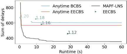
Before examining the experimental results in detail, we show the evolution of the solution in terms of the sum of delays for different algorithms on the same instance in Figure 2. Traditional algorithms, like EECBS, return a single solution, shown as a point. Anytime algorithms improve the solution as time progresses, shown as continuous curves. More details are provided in Experiment 6. To judge an anytime algorithm, we are interested in the Area Under the Curve (AUC) since it represents not only the sum of delays of the final solution but also how rapidly we approach it. We define AUC formally as the integral of the sum of delays graph, starting from the initial solution (since we only compare algorithms that start from the same initial solution), until the time limit is reached.
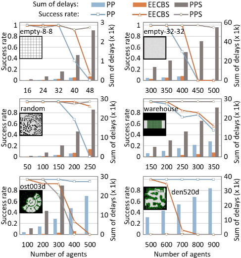
Experiment 1: Algorithms for initial planning. We compare three representative non-optimal algorithms in different categories for creating initial solutions, namely the boundedsuboptimal algorithm EECBS(2), the prioritized algorithm PP with a random priority ordering, and the rule-based algorithm PPS; all with a time limit of 10s. If an algorithm terminates before 10s without finding a solution, we restart it with a new random ordering of agents. As shown in Figure 3, no single algorithm dominates the other ones for all scenarios. However, the quality of the initial solution is usually not critical. With a poor initial solution, MAPF-LNS may take longer to converge, but the improvement is rapid. For example, when we run MAPF-LNS on the random map with 100 agents (using the parameters in Experiment 5) with initial solutions from EECBS, PP, and PPS, their initial sums of delays are very different, i.e., 299, 468, and 2,224, respectively, but their final sums of delays are close, i.e., 138, 141, and 136, respectively. The initial solution quality may be more important for harder instances since MAPF-LNS can then find it harder to improve the initial solutions. Hence, for each map and each number of agents, we use the algorithm with the highest success rate to find initial solutions in our future experiments.
Experiment 2: Algorithms for replanning. We test various types of algorithms for replanning paths, namely the prioritized algorithm PP with a random priority ordering, the bounded-suboptimal algorithm EECBS(1.1), and the optimal algorithm CBS (which always finds optimal solutions w.r.t. the chosen subset of agents, i.e., is guaranteed to reach the local minimum). We use the agent-based neighborhood heuristic with a neighborhood size of 4 to generate neighborhoods. Table 1 reports the resulting number of iterations, the sum of delays of the final solution, and the relative AUC w.r.t. PP. While CBS and, to a lesser extent, EECBS are competitive and occasionally even beat PP, overall PP is significantly better, dominating them on 74% of the tested instances in terms of AUC. This is because PP runs significantly faster than the other two algorithms and thus can explore a substantially larger number of neighborhoods within the time limit.
Experiment 3: Neighborhood selection heuristics. We compare MAPF-LNS using LNS with each of the three neighborhood selection heuristics discussed in Section 5 against MAPF-LNS using ALNS with all three heuristics. We use the same setting as in Experiment 2 and PP to replan. As shown in Table 2, different heuristics perform differently on different maps and different numbers of agents, but ALNS is overall the best one. While not always superior, it is at least the second best in each scenario and never more than 10% worse than the best heuristic in terms of AUC.
Experiment 4: Neighborhood sizes. We examine different neighborhood sizes N by trying alternate sizes of 2, 8, and 16, comparing to the size of 4 used up to this point. We use ALNS with the same setting as in Experiment 3. In general, larger neighborhoods have larger chances to find better solutions but require more time to replan, resulting in fewer iterations within the time limit. Table 3 shows that the neighborhood size makes a substantial difference, with larger neighborhood sizes being better for less congested instances.
Experiment 5: Solution quality. Table 4 shows the sum of delays of the initial and final solutions of MAPF-LNS using the same setting with the best neighborhood sizes as in Table 3. Within 60s, MAPF-LNS dramatically reduces the sum of delays by up to 36 times. Since most instances here are too hard for us to discover their optimal solutions, Table 4 reports an upperbound on the suboptimality of the final solution, namely the sum of costs of the final solution divided by the sum of costs of the individual shortest paths that ignore collisions with other agents. Overall, the suboptimality of MAPF-LNS is small. For the large maps (i.e., the warehouse, ost003d, and den520d maps), it is never worse than 14%, and almost certainly much better. For the small maps (i.e., the empty and randommaps), it can grow large for large numbers of agents, but the upperbound on the suboptimality is highly misleading since, for these extremely congested instances, the sum of costs of the optimal solution (if we could find it) is probably much larger than that of the individual shortest paths. When we use only instances for which we can find optimal solutions, the (actual) suboptimality of MAPFLNS is much smaller. Among the 750 (easier) instances used in Experiment 6, CBS solved 199 instances to optimality within 60s. Among these instances, MAPF-LNS finds optimal solutions for 171 instances and <0.01%, <0.1%, and <1% suboptimal solutions for 175, 195, and 198 instances, respectively. The worst solution is 1.35% suboptimal.
| In | m | Iterations (x 1k) | Final sum of delays | AUC | In | m | Iterations (x | Final sum of delays | AUC | |||||||||||
|---|---|---|---|---|---|---|---|---|---|---|---|---|---|---|---|---|---|---|---|---|
| P E | C | P | E | C | E P | C P | P | E | 1k) C | P | E | C | E P | C P | ||||||
| E | 16 | 1,644 | 257 | 275 | 3 | 3 | 3 | 1.00 | 1.03 | 300 | 68 | 36 | 22 | 437 | 435 | 1.28 | 1.31 | |||
| 24 | 1,125 | 170 | 131 | 13 | 13 | 13 | 1.00 | 0.98 | E | 350 | 45 | 27 | 17 | 450 879 | 855 | 1.03 | 1.02 | |||
| 32 | 1,013 | 125 | 98 | 30 | 32 | 31 | 1.04 | 1.03 | empty-32-32 | 400 | 29 | 18 | 11 | 855 1,616 | 1,614 | 1,593 | 1.01 | 1.02 | ||
| S | 40 | 1,319 | 104 | 86 | 76 | 80 | 71 | 1.15 | 1.10 | 450 | 11 | 1 | 1 | 6,588 | 26,991 | 28,544 | 1.72 | 1.72 | ||
| 48 | 770 | 32 | 20 | 1,067 | 834 | 969 | 0.88 | 0.98 | S | 500 | 3 | 1 | 1 | 37,013 | 47,055 | 47,233 | 1.13 | 1.13 | ||
| E | 50 | 206 | 60 | 30 | 27 | 28 | 27 | 1.05 | 1.01 | 150 | 13 | 10 | 3 | 132 | 136 | 133 | 1.06 | 1.06 | ||
| 100 | 71 | 32 | 16 | 143 | 147 | 142 | 1.03 | 0.98 | warehouse | E | 200 | 7 | 5 | 2 | 268 291 | 276 | 1.10 | 1.10 | ||
| 150 | 48 | 20 | 10 | 383 | 401 | 382 | 1.04 | 1.01 | 250 | 5 | 1 | 0.3 | 891 | 1,211 | 2,977 | 1.93 | 3.51 | |||
| 200 | 24 | 13 | 6 | 871 | 889 | 878 | 1.03 | 1.03 | S | 300 | 3 | 1 | 0.1 | 1,774 | 3,903 | 10,510 | 1.85 | 2.74 | ||
| S | 250 | 9 | 2 | 1 | 4,718 | 11,131 | 11,082 | 1.77 | 1.77 | 350 | 2 0.2 | 0.1 | 3,830 | 14,343 | 20,783 | 1.79 | 1.99 | |||
| P | 100 | 13 | 9 | 1 | 51 | 64 | 79 | 1.35 | 3.82 | 500 | 5 | 1 0.1 | 1,788 | 6,422 | 9,116 | 2.53 | 3.07 | |||
| 200 | 8 | 4 | 0.4 | 333 | 495 | 1,150 | 1.80 | 3.92 | 600 | 5 | 1 | 0.1 | 3,480 | 9,742 13,796 | 2.05 | 2.46 | ||||
| 300 | 7 | 2 | 0.2 | 1,198 | 2,139 | 4,806 | 1.75 | 2.95 | P | 700 | 5 | 0.3 | 0.1 5,980 | 15,743 | 18,678 | 1.88 | 2.04 | |||
| 400 | 5 | 1 | 0.1 | 3,337 | 7,217 | 10,344 | 1.78 | 2.11 | den520d | 800 | 4 | 0.3 | 0.1 10,149 | 21,003 | 24,008 | 1.55 | 1.67 | |||
| 500 | 3 | 0.3 | 0.1 | 8,813 | 15,171 | 17,969 | 1.43 | 1.54 | 900 | 4 | 0.4 | 0.1 15,275 | 27,133 | 30,371 | 1.40 | 1.49 | ||||
| m | Final Sum of delays | AUC | m | Final Sum of delays | AUC | |||||||||||
|---|---|---|---|---|---|---|---|---|---|---|---|---|---|---|---|---|
| Rand | Agent | Map | ALNS | Rand ALNS | Agent ALNS | Map ALNS | Rand | Agent | Map | ALNS | Rand ALNS | Agent ALNS | Map ALNS | |||
| empty-8-8 | 16 | 3 | 3 | 3 | 3 | 1.00 | 1.18 | 1.02 empty-32-32 | 300 | 453 | 437 | 418 | 408 | 1.11 | 1.06 | 1.01 |
| 24 | 12 | 13 | 13 | 12 | 0.99 | 1.12 | 1.08 | 350 | 853 | 852 | 794 | 772 | 1.10 | 1.08 | 1.02 | |
| 32 | 30 | 30 | 33 | 29 | 1.04 | 1.04 | 1.14 | 400 | 1,559 | 1,613 | 1,407 | 1,423 | 1.08 | 1.09 | 0.99 | |
| 40 | 83 | 76 | 85 | 74 | 1.16 | 1.04 | 1.11 | 450 | 4,626 | 7,774 | 5,618 | 4,469 | 0.96 | 1.31 | 1.18 | |
| 48 | 480 | 1,051 | 583 | 434 | 1.10 | 2.33 | 1.30 | 500 | 32,060 | 38,933 | 34,510 | 30,830 | 1.02 | 1.10 | 1.03 | |
| 50 | 25 | 27 | 28 | 25 | 0.99 | 1.06 | 1.07 | 150 | 138 | 134 | 146 | 130 | 1.11 | 1.03 | 1.19 | |
| 100 | 138 | 143 | 145 | 139 | 1.02 | 1.04 | 1.05 | 200 | 300 | 280 | 326 | 283 | 1.11 | 0.98 | 1.17 | |
| random 150 | 391 | 382 | 385 | 373 | 1.05 | 1.02 | warehouse 1.03 | 250 | 1,535 | 884 | 1257 | 831 | 1.41 | 1.09 | 1.53 | |
| 200 | 881 | 870 | 864 | 838 | 1.04 | 1.03 | 1.02 | 300 | 2,706 | 1,708 | 2,851 | 1,736 | 1.27 | 1.13 | 1.38 | |
| 250 | 3,388 | 4,700 | 3,843 | 3,988 | 0.90 | 1.13 | 1.01 | 350 | 4,555 | 3,694 | 6,917 | 3,256 | 1.14 | 1.11 | 1.28 | |
| 100 | 59 | 51 | 211 | 44 | 2.59 | 1.00 | 5.10 | 500 | 8,451 | 1,752 | 5,288 | 1,661 | 2.99 | 0.96 | 2.13 | |
| ost003d | 200 | 1,106 | 334 | 1,192 | 330 | 3.41 | 0.96 | den520d 3.08 1.81 | 600 | 13,087 | 3,415 | 7,669 | 3,462 | 2.31 | 0.94 | 1.64 |
| 300 | 3,964 | 1,215 | 2,985 | 1,227 | 2.46 | 0.92 | 700 | 17,364 | 6,209 | 11,024 | 6,597 | 1.82 | 0.93 | 1.37 | ||
| 400 | 8,779 | 3,289 | 5,777 | 3,343 | 1.92 | 0.96 | 1.42 | 800 | 22,607 | 9,882 | 14,969 | 10,054 | 1.61 | 0.95 | 1.25 | |
| 500 | 15,386 | 8,926 | 11,947 | 9,207 | 1.40 | 0.97 | 1.18 | 900 | 28,342 | 15,367 | 19,956 | 15,746 | 1.41 | 0.97 | 1.15 | |
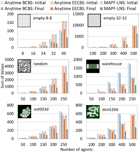
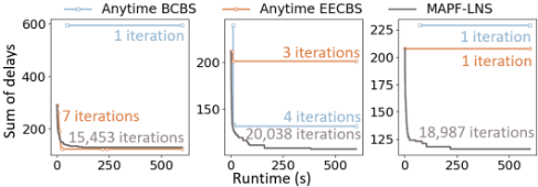
Experiment 6: Alternative anytime algorithms. We compare MAPF-LNS with the state-of-the-art anytime algorithm Anytime BCBS. Anytime BCBS is based on the bounded-suboptimal algorithm BCBS, which is much slower than more recent bounded-suboptimal algorithms, such as EECBS. We therefore also created an anytime version of EECBS based on restarting. Anytime EECBS starts with an initial suboptimality factor of 2. Whenever a solution with the sum of costs S is found, together with a lower bound L, the suboptimality factor is updated to 1 + 0.99 × (S/L - 1), and the search restarts. Since the value of S/L - 1 is guaranteed to be at least 1% smaller after each iteration, it will converge to 0 after a finite number of iterations. That is, the solutions of Anytime EECBS are guaranteed to converge to optimal. MAPF-LNS uses EECBS(2) to generate an initial solution (i.e., the same initial solution as used by Anytime EECBS), ALNS with a neighborhood size of 16 to generate neighborhoods, and PP to replan. Since Anytime BCBS and Anytime EECBS cannot find solutions for many of the instances used in our previous experiments, we use instances with fewer agents than before in this experiment. Table 5 summarizes the success rate, runtime to the initial solutions, and number of iterations, and Figure 4 summarizes the initial and final sums of delays. Since BCBS is slower than EECBS, Anytime BCBS has lower success rates and longer runtimes to the initial solution than the other two algorithms. Anytime BCBS and Anytime EECBS are essentially multiple runs of a bounded-suboptimal algorithm with decreasing suboptimality bounds, so they both result in exponentially longer iterations and thus fail to improve the initial solutions substantially. MAPF-LNS, on the other hand, focuses on a few (ideally highly-coupled) agents in each iteration and thus can perform substantially more iterations and improve the initial solution rapidly. Although the solutions of Anytime BCBS/EECBS are guaranteed to converge to optimal in theory [Cohen et al., 2018], this happens in practice only when the instances are very easy, such as some instances of the random and warehouse maps with 50 agents. MAPF-LNS does not have such guarantees, but its solutions also converge to optimal on most of those instances in practice. In addition, when facing harder instances that Anytime BCBS/EECBS cannot solve, MAPF-LNS can still solve them by using more efficient algorithms, such as PP and PPS, to find initial solutions and improve them over time.
| m | Iterations (x 1k) | AUC | m | Iterations (x 1k) | AUC | ||||||||||||
|---|---|---|---|---|---|---|---|---|---|---|---|---|---|---|---|---|---|
| N2 | N4 | N8 | N16 | N2 N4 | N8 N4 | N16 N4 | N2 | N4 | N8 | N16 | N2 N4 | N8 N4 | N16 N4 | ||||
| empty-8-8 | 16 | 3,268 | 1,548 | 832 | 510 | 1.25 | 0.97 | 0.97 | empty-32-32 | 300 | 172 | 87 | 33 | 17 | 1.18 | 0.92 | 0.99 |
| 24 | 2,708 | 1,455 | 800 | 451 | 1.39 | 0.89 | 0.88 | 350 | 117 | 55 | 20 | 10 | 1.15 | 0.98 | 1.11 | ||
| 32 | 2,558 | 1,236 | 655 | 381 | 1.38 | 0.91 | 0.87 | 400 | 71 | 33 | 13 | 6 | 1.09 | 1.00 | 1.17 | ||
| 40 | 2,727 | 1,593 | 809 | 431 | 1.71 | 0.91 | 1.84 | 450 | 27 | 15 | 3 | 1 | 1.19 | 1.54 | 1.85 | ||
| 48 | 1,971 | 1,363 | 226 | 52 | 1.12 | 3.59 | 4.20 | 500 | 5 | 4 | 1 | 0.4 | 1.04 | 1.13 | 1.19 | ||
| 50 | 451 | 257 | 146 | 81 | 1.11 | 0.96 | 0.95 | 150 | 28 | 19 | 11 | 6 | 1.22 | 0.95 | 0.89 | ||
| 100 | 206 | 103 | 49 | 28 | 1.10 | 0.94 | 0.94 | 200 | 14 | 9 | 5 | 2 | 1.13 | 0.94 | 0.93 | ||
| random 150 | 137 | 58 | 24 | 14 | 1.11 | 0.96 | 0.96 | warehouse 250 | 12 | 6 | 3 | 2 | 1.51 | 1.06 | 1.09 | ||
| 200 | 77 | 30 | 11 | 6 | 1.12 | 0.98 | 1.05 | 300 | 8 | 4 | 2 | 1 | 1.27 | 1.14 | 1.12 | ||
| 250 | 35 | 12 | 4 | 2 | 0.99 | 1.29 | 1.57 | 350 | 4 | 2 | 1 | 0.4 | 1.21 | 1.08 | 1.16 | ||
| 100 | 28 | 19 | 10 | 5 | 2.27 | 0.82 | 0.87 | 500 | 10 | 7 | 3 | 1 | 2.05 | 0.85 | 0.91 | ||
| 200 | 15 | 11 | 6 | 3 | 2.44 | 1.17 | 1.14 | 600 | 9 | 6 | 3 | 1 | 1.77 | 0.85 | 0.83 | ||
| ost003d 300 | 11 | 7 | 3 | 1 | 1.81 | 1.00 | 0.97 | den520d 700 | 8 | 5 | 2 | 1 | 1.53 | 0.83 | 0.81 | ||
| 400 | 8 | 5 | 2 | 1 | 1.66 | 0.90 | 0.95 | 800 | 7 | 5 | 2 | 1 | 1.43 | 0.83 | 0.85 | ||
| 500 | 5 | 3 | 1 | 0.4 | 1.31 | 0.97 | 1.02 | 900 | 6 | 4 | 2 | 1 | 1.31 | 0.91 | 0.84 | ||
| N | m | Sum of delays | Sub- | N | m Sum of delays | Sub- opt | N | m | Sum of | delays | Sub- | ||||||
|---|---|---|---|---|---|---|---|---|---|---|---|---|---|---|---|---|---|
| Initial | Final | opt | Initial | Final | Initial | Final | opt | ||||||||||
| empty-8-8 | 16 | 16 | 7 | 3 | ≤1.03 | 8 | 300 1,515 | 367 | ≤1.06 | random | 16 | 50 | 47 | 24 | ≤1.02 | ||
| 16 | 24 | 33 | 11 | ≤1.09 | 8 | 350 2,740 | 743 | ≤1.10 | 16 | 100 | 299 | 130 | ≤1.06 | ||||
| 16 | 32 | 79 | 25 | ≤1.16 | 8 | 400 4,445 | 1,374 | ≤1.16 | 16 | 150 | 914 | 346 | ≤1.10 | ||||
| 8 | 40 | 1,314 | 63 | ≤1.30 | empty-32-32 | 4 | 450 40,513 | 5,121 | ≤1.54 | 8 | 200 | 2,139 | 792 | ≤1.18 | |||
| 4 | 48 | 2,586 | 668 | ≤3.67 | 4 | 500 55,057 | 33,554 | ≤4.16 | 4 | 250 | 24,455 | 3,390 | ≤1.60 | ||||
| warehouse | 16 | 150 | 261 | 124 | ≤1.01 | ost003d | 8 | 100 1,338 | 37 | ≤1.00 | den520d | 8 | 500 | 12,002 | 869 | ≤1.01 | |
| 16 | 200 | 526 | 266 | ≤1.02 | 4 | 200 4,103 | 346 | ≤1.01 | 8 | 600 | 16,424 | 2,034 | ≤1.02 | ||||
| 8 | 250 | 13,199 | 635 | ≤1.03 | 8 | 300 8,129 | 1,098 | ≤1.02 | 16 | 700 | 20,713 | 4,473 | ≤1.04 | ||||
| 8 | 300 | 18,587 | 1,400 | ≤1.06 | 8 | 400 13,634 | 2,427 | ≤1.04 | 8 | 800 | 25,885 | 7,408 | ≤1.05 | ||||
| 4 | 350 | 25,539 | 3,979 | ≤1.14 | 8 | 500 19,914 | 8,223 | ≤1.11 | 16 | 900 | 31,888 | 12,186 | ≤1.08 | ||||
| m | Success rate | Time to sol | Iterations | Success rate | Time to sol | Iterations | |||||||||||
|---|---|---|---|---|---|---|---|---|---|---|---|---|---|---|---|---|---|
| B LNS | B LNS | B E | LNS | m | B LNS | B LNS | B | E | LNS | ||||||||
| empty-8-8 | 8 | 1.00 | 1.00 | 0.0002 | 0.0002 | 1 | 2 | 1,053k | empty-32-32 | 100 | 1.00 | 1.00 | 0.05 0.02 | 10 | 7 | 111k | |
| 16 | 1.00 | 1.00 | 0.0012 | 0.0005 | 2 | 4 | 524k | 200 | 1.00 | 1.00 4.21 | 0.11 | 15 | 7 | 55k | |||
| 24 | 1.00 | 1.00 | 0.01 | 0.0018 | 8 | 11 | 462k | 300 | 0.72 | 1.00 16.96 | 0.45 | 8 | 5 | 18k | |||
| 32 | 1.00 | 1.00 | 0.05 | 0.01 | 7 | 11 | 377k | 400 | 0.00 | 1.00 - | 3.36 | - | 4 | 7k | |||
| 40 | 0.60 | 1.00 | 0.87 | 0.43 | 5 | 4 | 401k | 500 | 0.00 | 1.00 - | 33.33 | - | 1 | 1k | |||
| 50 | 1.00 | 1.00 | 0.06 | 0.02 | 17 | 10 | 78k | warehouse | 50 | 1.00 | 1.00 0.23 | 0.03 | 3 | 3 | 13k | ||
| 100 | 0.96 | 1.00 | 0.88 | 0.10 | 11 | 8 | 27k | 100 | 0.92 | 1.00 1.54 | 0.12 | 23 | 8 | 12k | |||
| random 150 | 0.88 | 1.00 | 9.63 | 0.42 | 7 | 6 | 13k | 150 | 0.92 | 1.00 7.65 | 0.90 | 17 | 5 | 6k | |||
| 200 | 0.08 | 1.00 | 39.60 | 1.50 | 2 | 6 | 6k | 200 | 0.80 | 1.00 27.00 | 2.86 | 4 | 3 | 3k | |||
| 250 | 0.00 | 1.00 | - | 5.00 | - | 4 | 4k | 250 | 0.28 | 1.00 33.04 | 4.67 | 6 | 2 | 2k | |||
| 50 | 1.00 | 1.00 | 0.30 | 0.06 | 2 | 5 | 7k | 100 | 0.92 | 1.00 0.69 | 0.26 | 2 | 4 | 5k | |||
| 100 | 0.92 | 1.00 | 2.42 | 0.22 | 6 | 6 | 5k | 200 | 0.68 | 1.00 4.35 | 0.88 | 5 | 5 | 3k | |||
| ost003d 150 | 0.84 | 1.00 | 6.98 | 1.48 | 4 | 4 | 3k | den520d | 300 | 0.44 | 1.00 12.39 | 1.83 | 3 | 3 | 2k | ||
| 200 | 0.52 | 1.00 | 18.20 | 1.86 | 2 | 3 | 2k | 400 | 0.08 | 1.00 20.98 | 3.16 | 1 | 2 | 2k | |||
| 250 | 0.16 | 1.00 | 29.72 | 2.88 | 3 | 1 | 2k | 500 | 0.00 | 1.00 - | 3.58 | - | 1 | 1k | |||
Experiment 7: Longer time limits. To better understand the anytime behavior of the three algorithms, we repeat previous experiments with a time limit of 600s on map den520d. The final sums of delays of MAPF-LNS are usually smaller (by at most 12%), but the trends are the same (i.e., PP is the best replanning algorithm, and ALNS works better than LNS). Anytime BCBS and Anytime EECBS, on the other hand, run out of memory in many cases. Moreover, their final sums of delays and numbers of iterations do not change much, and their AUC graphs usually become flat after a few seconds (see Figure 5). Similar memory issues of CBS-based algorithms have been observed in [Boyarski et al., 2020], and similar convergence behavior of Anytime BCBS has been observed in [Cohen et al., 2018].
Experiment 8: Train planning. We have recently applied MAPF-LNS to the 2020 Flatland Challenge, a NeurIPS competition about planning collision-free paths for trains on rail networks [Laurent et al., 2021]. We won both rounds of the competition, and MAPF-LNS was an essential algorithm in our software which helped to improve our score by 0.010 (= 3 times the difference to the team in second place) in Round 1 and 0.709 (= 61% the difference to the team in second place) in Round 2. More details can be found in [Li et al., 2021b].
8 Conclusions
In this work, we demonstrated that the use of Large Neighborhood Search (LNS) leads to very scalable and high-quality solutions to MAPF and significantly outperforms existing anytime algorithms in terms of success rates, runtimes to the first solution, and speed of improving the solution. We performed extensive experiments with a variety of algorithms. On easy instances that the optimal algorithm CBS can solve within 60s, our algorithm MAPF-LNS also finds optimal solutions in most cases, within 1.35% of optimal in the worst case. On harder instances that the bounded-suboptimal algorithm EECBS can solve, MAPF-LNS rapidly improves the solution found by EECBS to near-optimal. On very challenging instances that only the unbounded-suboptimal algorithms PPS or PP can solve, MAPF-LNS rapidly reduces the sum of delays of the solution found by PPS or PP by up to 36 times.
Acknowledgments
We thank Keisuke Okumura for providing us his PPS implementation. The research at the University of Southern California was supported by the National Science Foundation under grant numbers 1409987, 1724392, 1817189, 1837779, and 1935712 as well as a gift from Amazon. The research at Monash University was partially supported by the Australian Research Council under Discovery Grants DP190100013 and DP200100025 as well as a gift from Amazon.
@inproceedings{ijcai2021p568,
  title     = {Anytime Multi-Agent Path Finding via Large Neighborhood Search},
  author    = {Li, Jiaoyang and Chen, Zhe and Harabor, Daniel and Stuckey, Peter J. and Koenig, Sven},
  booktitle = {Proceedings of the Thirtieth International Joint Conference on
               Artificial Intelligence, {IJCAI-21}},
  publisher = {International Joint Conferences on Artificial Intelligence Organization},
  editor    = {Zhi-Hua Zhou},
  pages     = {4127--4135},
  year      = {2021},
  month     = {8},
  note      = {Main Track},
  doi       = {10.24963/ijcai.2021/568},
  url       = {https://doi.org/10.24963/ijcai.2021/568},
}
TY - CPAPER TI - Anytime Multi-Agent Path Finding via Large Neighborhood Search AU - Li, Jiaoyang AU - Chen, Zhe AU - Harabor, Daniel AU - Stuckey, Peter J. AU - Koenig, Sven T2 - Proceedings of the Thirtieth International Joint Conference on Artificial Intelligence, IJCAI-21 PB - International Joint Conferences on Artificial Intelligence Organization PY - 2021 SP - 4127 EP - 4135 DO - 10.24963/ijcai.2021/568 UR - https://doi.org/10.24963/ijcai.2021/568 ER -Copied
Machine-readable versions of this paper, for tools and AI agents:





