
Parallel Subtrajectory Alignment over Massive-Scale Trajectory Data
Proceedings of the Thirtieth International Joint Conference on Artificial Intelligence. Main Track. Pages 3613-3619.
https://doi.org/10.24963/ijcai.2021/497
© 2021 International Joint Conferences on Artificial Intelligence
Keywords
- Multidisciplinary Topics and Applications: Transportation
- Data Mining: Mining Spatial, Temporal Data
Abstract
We study the problem of subtrajectory alignment over massive-scale trajectory data. Given a collection of trajectories, a subtrajectory alignment query returns new targeted trajectories by splitting and aligning existing trajectories. The resulting functionality targets a range of applications, including trajectory data analysis, route planning and recommendation, ridesharing, and general location-based services. To enable efficient and effective subtrajectory alignment computation, we propose a novel search algorithm and filtering techniques that enable the use of the parallel processing capabilities of modern processors. Experiments with large trajectory datasets are conducted for evaluating the performance of our proposal. The results show that our solution to the subtrajectory alignment problem can generate high-quality results and are capable of achieving high efficiency and scalability.
- [Chen et al., 2010] Zaiben Chen, Heng Tao Shen, Xiaofang Zhou, Yu Zheng, and Xing Xie. Searching trajectories by locations: an efficiency study. In SIGMOD, pages 255- 266, 2010.
- [Chen et al., 2019] Lisi Chen, Shuo Shang, Christian S. Jensen, Bin Yao, Zhiwei Zhang, and Ling Shao. Effec- tive and efficient reuse of past travel behavior for route recommendation. In KDD, 2019.
- [Chen et al., 2020] Lisi Chen, Shuo Shang, and Tao Guo. Real-time route search by locations. In AAAI, pages 574- 581, 2020.
- [Dijkstra, 1959] E. W. Dijkstra. A note on two problems in connection with graphs. Numerische Math, 1:269-271, 1959.
- [Driemel et al., 2020] Anne Driemel, Petra Mutzel, and Lutz Oettershagen. Spatio-temporal top-k similarity search for trajectories in graphs. CoRR, abs/2009.06778, 2020.
- [Frentzos et al., 2007] E. Frentzos, K. Gratsias, and Y. Theodoridis. Index-based most similar trajectory search. In ICDE, pages 816-825, 2007.
- [Liu et al., 2014] Kuien Liu, Yaguang Li, Jian Dai, Shuo Shang, and Kai Zheng. Compressing large scale urban tra- jectory data. In CloudDP@EuroSys, pages 3:1-3:6. ACM, 2014.
- [Liu et al., 2016] Jiajun Liu, Kun Zhao, Philipp Sommer, Shuo Shang, Brano Kusy, Jae-Gil Lee, and Raja Jurdak. A novel framework for online amnesic trajectory compres- sion in resource-constrained environments. IEEE Trans. Knowl. Data Eng., 28(11):2827-2841, 2016.
- [Shang et al., 2012] Shuo Shang, Ruogu Ding, Bo Yuan, Kexin Xie, Kai Zheng, and Panos Kalnis. User oriented trajectory search for trip recommendation. In EDBT, pages 156-167, 2012.
- [Shang et al., 2014] Shuo Shang, Ruogu Ding, Kai Zheng, Christian S. Jensen, Panos Kalnis, and Xiaofang Zhou. Personalized trajectory matching in spatial networks. VLDB J., 23(3):449-468, 2014.
- [Shang et al., 2017] Shuo Shang, Lisi Chen, Zhewei Wei, Christian S. Jensen, Kai Zheng, and Panos Kalnis. Tra- jectory similarity join in spatial networks. PVLDB, 10(11):1178-1189, 2017.
- [Xie et al., 2017] Dong Xie, Feifei Li, and Jeff M. Phillips. Distributed trajectory similarity search. Proc. VLDB En- dow., 10(11):1478-1489, 2017.
- [Yuan and Li, 2019] Haitao Yuan and Guoliang Li. Dis- tributed in-memory trajectory similarity search and join on road network. In ICDE, pages 1262-1273, 2019.
- [Yuan et al., 2013] Jing Yuan, Yu Zheng, Xing Xie, and Guangzhong Sun. T-drive: Enhancing driving directions with taxi drivers' intelligence. IEEE Trans. Knowl. Data Eng., 25(1):220-232, 2013.
- [Zhao et al., 2018] Yan Zhao, Shuo Shang, Yu Wang, Bo- long Zheng, Quoc Viet Hung Nguyen, and Kai Zheng. REST: A reference-based framework for spatio-temporal trajectory compression. In Yike Guo and Faisal Farooq, editors, KDD, pages 2797-2806, 2018.
- [Zheng et al., 2013] Kai Zheng, Shuo Shang, Nicholas Jing Yuan, and Yi Yang. Towards efficient search for activity trajectories. In ICDE, pages 230-241, 2013.
- [Zheng et al., 2017] Kai Zheng, Bolong Zheng, Jiajie Xu, Guanfeng Liu, An Liu, and Zhixu Li. Popularity-aware spatial keyword search on activity trajectories. World Wide Web, 20(4):749-773, 2017.
- [Zheng et al., 2018] Bolong Zheng, Haozhou Wang, Kai Zheng, Han Su, Kuien Liu, and Shuo Shang. Sharkdb: an in-memory column-oriented storage for trajectory anal- ysis. World Wide Web, 21(2):455-485, 2018.
References were extracted automatically from the PDF and may contain errors.
Full text extracted automatically from the PDF; figures, tables and equations may differ. The PDF is the version of record.
1 Introduction
With the continued proliferations of GPS-enabled devices (e.g., smartphones, vehicle navigation systems, wearable smart devices) and online location-based services (e.g., Uber, Lyft, Google Maps), trajectory data is being generated at an unprecedented scale. For example, the average number of for-hire vehicle trips per day from New York City during the first half of year 2020 is well over 400K. 1 The availability of massive-scale trajectory data enables trajectory similarity search [Chen et al., 2010; Driemel et al., 2020; Xie et al., 2017; Yuan and Li, 2019; Shang et al., 2014], which finds trajectories that are similar in some specific sense to a set of query locations. Trajectory similarity search is one of the fundamental problems in spatio-temporal data analytics. It has a broad range of applications, including indepth trajectory data explorations, ridesharing service analytics, route planning and recommendations for energy saving and emission reduction, and other location-based services.
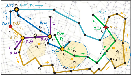
Given a collection of trajectory data D, existing studies formulate the trajectory similarity search problem as a query that finds a subset of D based on spatial (i.e., proximity to query locations) and temporal (i.e., travel time interval) constraints. However, it is likely that the quality of query results fails to meet users' expectation due to data sparsity, especially when a user defines a very stringent spatio-temporal constraint (i.e., a narrow time interval, a high similarity threshold). Consider a toy example in Figure 1, where vs and ve, denoted by red pentagon and star, respectively, are source and destination locations, O = {o1, o2, o3} are query locations, T = [8:30,9:30] denotes the query constraint of travel time interval. Let τ1 (yellow), τ2 (dark blue), τ3 (green), τ4 (purple), and τ5 (light blue) be five trajectories in D. Traditional trajectory similarity search aims to find trajectories that are spatially and temporally close to the query. In this example, we may find that τ1 is the only trajectory that meets departure (vs), destination (ve), and time interval ([8 : 30, 9 : 30]) requirements. However, this result may not be good enough in real applications like ridesharing recommendations because τ1 is not close enough to query locations. Additionally, if a user set a stringent requirement on similarity threshold, it is very likely that no trajectory in D meets query requirements.
∗Corresponding author.
1 https://data.cityofnewyork.us/browse?q=trip
In this light, we study a novel problem of Sub-Trajectory Alignment (STA) over a collection of trajectory data D. The STA problem not only considers existing trajectories in D, but also generates and evaluates new trajectories by splitting and aligning exiting trajectories in D. Specifically, given source and destination locations, vs and ve, respectively, a set of query locations O, a travel time interval T = [ts, te], a similarity threshold θ, the maximum number of sub-trajectory alignments M, the STA problem finds all existing trajectories in D and all trajectories generated by sub-trajectory alignments from D such that: (1) Each result trajectory τr covers vs and ve and the arrival timestamps regarding vs and ve are within T ; (2) The similarity between τr and O is no less than θ; (3) Trajectory τr is generated from the alignment of at most M +1 existing trajectories fromD. Consider the example in Figure 1, we may derive two feasible trajectories by aligning two existing trajectories: τr1 = vs → τ2 → v0 → τ5 → ve; τr2 = vs → τ2 → v3 → τ3 → ve. Compared to the original result trajectory τ1, τr2 is more similar (closer) to query locations o1, o2, and o3. Thus, we may acquire results with higher quality by aligning only two existing trajectories.
It is challenging to answer the STA problem efficiently. Given query location set O, we have ∑Mi=0 S(|O|, i + 1) different partitionings where S(·, ·) denotes the Stirling number of the second kind. Thus, it is computationally prohibitive to enumerate and evaluate all possible location partitionings. To address the challenge, we develop Parallel Sub-Trajectory Alignment Search (PSTAS) algorithm for answering the STA problem. The high-level idea of PSTAS works as follow. Let q be an STA query, which consists of source location vs, destination location ve, a set of query locations O, travel time interval T = [ts, te], similarity threshold θ, and the maximum number of sub-trajectory alignments M. The PSTAS has two phases: (1) Generation of trajectory candidates through network expansion; (2) Alignment of trajectory candidates through bottom-up merging.
Initially, we regard vs, ve, and each location in O as individual network expansion centers. We run Dijkstra's Algorithm [Dijkstra, 1959] to explore the road network and to find trajectory candidates that are close to each expansion center. Here, we propose a pruning technique to filter out unqualified candidates at an early stage. Note that the expansions from different locations are independent of each other so they can be executed in parallel.
Next, we generate partitionings of the set O. Each partitioning contains k disjoint expansion center sets (k ∈ [1, M+ 1]). For each expansion center set in each partitioning, we evaluate and merge the trajectory candidates associated with the expansion center. For each partitioning, we merge the candidates associated with each expansion center set in a bottom-up fashion. The computations in each group and in each partitioning occur in parallel. Similarly, the computations in different partitionings are independent of each other so they are capable of running in parallel.
Our contributions are summarized as follows. First, we define and study a novel problem of Sub-Trajectory Alignment (STA), aiming to address the limitation of low result quality for traditional trajectory similarity search with insufficient trajectory data. Second, we develop a PSTAS algorithm that is capable of answering the STA problem efficiently. Third, we conduct extensive experiments on large trajectory data. The experiment results confirm that: (1) Answering the STA problem is substantially more likely to find high-quality trajectory results in comparison to answering existing trajectory similarity search problem; (2) Our PSTAS algorithm is capable of answering the STA problem over a collection of up to 10M trajectories with user interaction time.
2 Preliminaries and ProblemDefinition
2.1 Road Network and Trajectory
We formulate a road network by a connected and undirected graph G = (V,E, F,W), where V denotes a set of vertices and E ⊆ {{vi, vj}|vi, vj ∈ V ∧ vi ̸= vj} denotes a set of edges. Here, a vertex v ∈ V denotes a road intersection or endpoint, an edge e = {vi, vj} ∈ E denotes a road segment. Function F : V ∪ E → Geometries denotes the following two mapping operations: (1) Mapping a vertex to the point location (road intersection or endpoint); (2) Mapping an edge to a polyline that represents the corresponding road segment. Function W : E → R assigns a weight W(e) to an edge e, which denotes the corresponding road segment's length. For simplicity, we assume that the location points are located on vertices.
This modeling of road networks aligns with previous studies (e.g. [Chen et al., 2010; Shang et al., 2014]). Trajectory and sub-trajectory are defined as follow.
Definition 1 (Trajectory) Trajectory τ is a sequence of vertex-timestamp pairs 〈p1, p2, ..., pn〉. Note that pi = (vi, ti) where vi represents the vertex and ti denotes the timestamp when τ passes vi.
Definition 2 (Sub-trajectory) A sub-trajectory of τ, denoted by τ(pi → pj), is a segment of τ, where pi, pj ∈ τ and pi and pj are the start and end vertex-timestamp pairs of the segment, respectively.
2.2 ProblemFormulation
Definition 3 (Valid Sub-Trajectory Alignment) Given a source location vs, a destination location ve, a time interval T = [ts, te], and a collection of trajectories D, a valid sub-trajectory alignment, denoted by 〈τ1(p1 → p2), τ2(p2 → p3), ..., τn(pn → pn+1)〉, satisfies the following conditions: (1) n ≥ 2; (2) τi ∈ D (i ∈ [1, n]); (3) p1 = (vs, t1) where t1 ≥ ts; (4) pn+1 = (ve, tn+1) where tn+1 ≤ te.
Definition 4 (Sub-Trajectory Alignment (STA) Problem) Given a collection D of trajectories, the STA problem takes the following arguments as input: (1) Source and destination locations, vs and ve, respectively, and a set of query locations O; (2) A travel time interval T = [ts, te]; (3) A similarity threshold θ; (4) The maximum number of subtrajectory alignments M. The STA problem finds all valid sub-trajectory alignments R such that: (1) The similarity between O and each sub-trajectory alignment τr ∈ R, denoted by Sim(O, τr), is no less than θ (i.e., Sim(O, τr) ≥ θ); (2) The number of sub-trajectories in each alignment does not exceed M.
2.3 SimilarityMeasures
Given a location v and a trajectory τ, the proximity d(v, τ) between v and τ is defined by Equation 1.
where dmin(v, vi) denotes the shortest network distance between v and vi. Given a set O of locations and a trajectory
τ, the similarity Sim(O, τ) between them is defined by the aggregate distance [Chen et al., 2010; Shang et al., 2017]:
3 Parallel Subtrajectory Alignment Search
Our PSTAS algorithm consists of two phases: (1) Generation of trajectory candidates (Section 3.1); (2) Alignment of subcandidates (Section 3.2).
3.1 Generating Trajectory Candidates
This section presents our algorithm details regarding how to generate trajectory candidates associated with each location. Specifically, we present how to generate trajectory candidates associated with vs, ve, and each location in O, respectively. Trajectory candidates are potentially capable for alignment. To generate trajectory candidates associated with vs and ve, we retrieve all trajectories that pass vs after ts, and retrieve all trajectories that pass ve before te. To generate trajectory candidates associated with each location in O (i.e., o1, o2, o3, and o4), we perform network expansion from each location based on Dijkstra's algorithm [Dijkstra, 1959].
We terminate the network expansion from each location oi when we are unable to find potentially qualified trajectory for alignment through further network expansion. As such, we pre-identify a network expansion region ri for each location oi. Region ri is a circle in network space. The center of ri is oi and the radius is the network distance from oi to the expansion boundary. From Figure 1, we see that the expansion boundaries of o1, o2, and o3 are illustrated by light yellow areas. Note that Dijkstra's algorithm iteratively selects the vertex from road networks with the minimum distance label for expansion. As such, given a trajectory τ, if pm.vm (pm ∈ τ) is the first vertex visited by the expansion from oi, vm is the vertex nearest to oi. It is worthy of noting that expansions from different locations are independent of each other. Thus, they can be performed in parallel.
Given an expansion center oi, we proceed to present how to determine the radius of its expansion region ri. Specifically, if a vertex v is visited during the Dijkstra's expansion from oi and trajectory τ covers v, we calculate the similarity upper bound between O and τ, denoted by Sim⊤oi (O, v), based on Equation 3.
During the process of network expansion from oi, if Sim⊤oi (O, v) < θ, we terminate the expansion from oi because all unvisited trajectories so far are unqualified for alignment. As shown in Figure 1, when we run network expansion from o1, we retrieve τ1 and τ4 as trajectory candidates because both trajectories spatially overlap with o1's expansion region. Likewise, we retrieve τ2 and τ3 as trajectory as candidates associated with o2, and retrieve τ1 and τ3 as candidates associated with o3.
Data structure. During the expansion process, we maintain a candidate set S(o) for expansion center o, including vs, ve, and all oi ∈ O. Each trajectory candidate τ in S(o) is represented by a trajectory label, denoted by lo(τ, vp) = 〈e, vp, d〉, where e is the entry of τ , vp denotes the vertex covered by τ that is visited during the network expansion from o, and d denotes the network distance from vp to o.
Algorithm for generating trajectory candidates. Algorithm 1 presents the pseudo code for generating trajectory candidates associated with vs, ve, and each location oi ∈ O. The inputs are start and end locations (vs and ve), locations O, similarity threshold θ, and travel time interval T. The output is trajectory candidate sets of vs, ve, and each location in O (i.e., S = {S(vs), S(ve), S(o1), ..., S(o|O|)}). In particular, each S(·) ∈ S is indexed by a min-heap consisting of trajectory labels associated with each location. Trajectory labels in S(o) are sorted in ascending order of lo(τ, vp).d (i.e., the network distance between o and vp). First, we initialize the result trajectory candidate set associated with vs, ve, and each oi ∈ O (lines 1-2). Next, we find trajectory candidates associated with vs and ve respectively (lines 3-10). Specifically, we first evaluate all trajectories that cover vs. For each trajectory τ, we add τ into vs's candidate pool if τ passes vs after T.ts (lines 5-6). Likewise, we proceed to evaluate all trajectories that cover ve. For each trajectory τ, we add τ into ve's candidate pool if τ passes vs before T.te (lines 9-10). Next, we perform a Dijkstra's Algorithm based network expansion from eachinte location oi ∈ O. We iteratively retrieve the next vertex that has not been scanned (line 12). Then we compute the upper bound of similarity between O and trajectories covering vp (i.e., simub i ) (line 14). If simub i ≥ θ, we insert the labels of trajectories that cover vp to S(oi) (lines 16-17); Otherwise, we terminate the expansion process.
3.2 Alignment of Trajectory Candidates
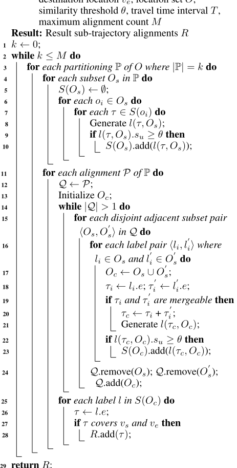
Having trajectory candidates of vs, ve, and O, we need to find qualified alignment of these trajectory candidates. Our high-level idea works as follow. First, we derive all qualified partitionings for location set O. Each qualified partitioning, denoted by P (|P| ≤ M), is a set of disjoint location subsets Os of O, and the union of these subsets is O. Second, for each partitioning we generate trajectory candidates associated with each location subset Os ∈ P. Finally, based on those trajectory candidates, we generate qualified sub-trajectory alignments regarding each possible partitioning.
We present the data structure we used for processing trajectory candidate alignment. In order to represent and index each trajectory candidate associated with each location subset Os ∈ P, we maintain a subset trajectory candidate label of each trajectory τ associated with each location subset Os. The label is denoted by l(τ,Os) = 〈e,H, su〉 where e is the entry of τ , H is a hashmap where keys are locations in Os and values are their corresponding vertices visited by the expansion algorithm, and su denotes the upper bound of similarity between O and τ , which is computed by Equation 4.
Algorithm 1: TrajCandidatesGen
Data: Start location vs, end location ve, query location set O, similarity threshold θ, travel time interval T Result: S = {S(vs), S(ve), S(o1), ..., S(o|O|)} 1 for each S(·) in S do 2 S(·) ←∅; 3 for each trajectory τ that covers vs do 4 p ←τ.p1; 5 if p.t1 is after T.ts then 6 S(vs).add(lvs (τ, vs)); 7 for each trajectory τ that covers ve do 8 p ←τ.p|τ|; 9 if p.t|τ| is before T.te then 10 S(ve).add(lve (τ, ve)); 11 for each location oi ∈ O do 12 while NetworkExpansion(oi).hasNext() do 13 vp ←NetworkExpansion(oi).next(); 14 simub i ← |O| + e-dmin(oi,vp) -1; 15 if simub i ≥ θ then 16 for each τ that covers vp do 17 S(oi).add(loi (τ, vp)); 18 else 19 break; 20 return S;where vp denotes the vertex visited by the network expansion from oi.
Algorithm of alignment. Algorithm 2 presents the pseudo code of trajectory alignment. We evaluate each qualified partitioning P of O where the number of subsets ranges from 1 to M. For each location subset Os ∈ P we evaluate trajectory candidates associated with each oi ∈ Os and derive trajectory candidates associated with Os (lines 4-10). For each qualified trajectory candidate of Os, we generate and index its label (lines 9-10). Next, we merge all subset trajectory candidates in a bottom-up manner. We evaluate each alignment (sequence) of subsets P, denoted by Q, by merging candidates from adjacent subsets hierarchically (lines 1128). Specifically, given an adjacent subset pair 〈Os,O′s 〉 we evaluate each indexed subset trajectory candidate pair, τi and τ ′ i , and check if they are mergeable (lines 19-21). In particular, τi and τ ′ i are mergeable if they have intersection vertex and their arrival timestamps on the intersection vertex meet temporal alignment requirement. If they are mergeable, we generate the label for τc, which is an aligned trajectories of τi and τ ′ i (lines 22-23). Next, we update Q by merging Os and O′s (line 24). The merging process terminates when Q only has one set. Upon termination, we have generated labels associated with the entire location set. Here, we add all trajectories that cover vs and ve into the result pool.
Algorithm 2: TrajAlignment
Data: Trajectory candidate sets S, source location vs, destination location ve, location set O,
4 Experiments
4.1 Experiment Settings
Datasets. We apply the following two road networks: Beijing Road Network (BN) and the New York Road Network (NYN) 2 . BN consists of ∼28K vertices and ∼27K edges. NYN consists of ∼95K vertices and ∼261K edges. For BN, we use taxi trajectory data collected by the T-drive project [Yuan et al., 2013], which consists of 800K trajec- Ratio of Qualified Results tories. For NYN, we use taxi trip data from New York 3 , which consists of 800M trips. Note that each taxi trip from New York only contains pick-up and drop-off locations and timestamps. As such, we generate a trajectory by deriving the shortest network path from the pick-up location to the dropoff location.
2 https://lab-work.github.io/data/
Implementations. The road networks, trajectories, and indices are memory resident. All algorithms are implemented in Java and run on a server with two Intel® Xeon® Processors Gold 5120 and 64GB RAM. Unless stated otherwise, experiment results are averaged over 100 independent trials using different vs, ve, and O for efficacy and efficiency evaluations.
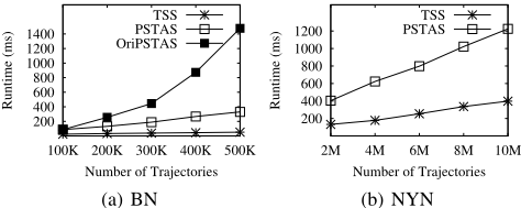
Baselines. We evaluate the following methods. (1) Trajectory Similarity Search without Alignment (TSS): Given a collection of trajectories, TSS returns a set of existing trajectories satisfying the similarity and temporal requirements. Note that TSS is equivalent to PSTAS where M = 0. (2) Parallel Sub-Trajectory Alignment Search (PSTAS): Algorithm 1 and Algorithm 2. (3) PSTAS without Pruning Technique (OriPSTAS): PSTAS without calculating the similarity upper bound for filtering unqualified trajectory candidates at an early stage.
Evaluationmetrics. We use the followingmetrics to evaluate the effectiveness and efficiency of each method. (1) Ratio of qualified results: Given N independent trials, let Nq be the number of trials that return at least one qualified trajectory alignment. The ratio of qualified results is defined by Nq N . (2) Runtime: The average time cost of query processing. The parameter settings are listed in Table 1.
3 https://data.cityofnewyork.us/browse?q=trips
Ratio of Qualified Results
Runtime (ms)
Ratio of Qualified Results
TSS
PSTAS
OriPSTAS
0.6
0.7
0.8
0.9
Similarity Threshold
(a) BN
| BN | NYN | |
|---|---|---|
| Number of trajecto- ries | 100K-500K / de- fault 300K | 2M-10M / de- fault 2M |
| Maximum number of alignments M | 1-3 / default 2 | 1-3 / default 2 |
| Number of intermedi- ate locations |O| | 3-7 / default 5 | 3-7 / default 5 |
| Similarity threshold θ | 0.60-0.90 / default 0.80 | 0.80-0.95 / de- fault 0.90 |
| Travel time interval T | randomly gener- ated from 0.5 to 3 hours | randomly gener- ated from 0.5 to 3 hours |
| Thread count | 16-48 / default 48 | 16-48 / default 48 |
4.2 Experiment Results
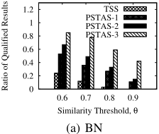
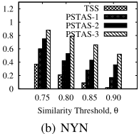
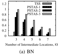
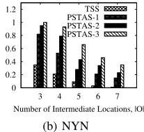
Varying similarity threshold (effectiveness). First, we evaluate the ratio of individual trails that return qualified trajectories. We vary the similarity threshold θ on BN and NYN. In Figure 2, the "x" from "PSTAS-x" denotes the value of M. As we increase the similarity threshold, all methods exhibit a decreasing trend regarding the ratio of results with qualified trajectories. PSTAS-x performs consistently better than TSS. In particular, when we let θ be 0.8 in BN, TSS only has 3% trails (queries) that return qualified trajectories. When we increase θ to 0.9, none of the trails find qualified trajectories. In contrast, PSTAS-1, PSTAS-2, and PSTAS-3 have 27%, 33%, and 59% trails that return qualified results, respectively, when we set θ to 0.8. Such contrast clearly demonstrates that PSTAS, even with a small number of trajectory alignments, is substantially more likely to find high-quality results (i.e.,
500
400
300
200
100
trajectories that are highly similar to query locations) than traditional trajectory similarity search method.
Varying the number of locations (effectiveness). Next, we evaluate the ratio of individual trails that return qualified trajectories as we vary the number of intermediate locations (|O|). From Figure 3, we see that all methods perform worse as we increase the number of intermediate locations.
Varying the number of trajectories. This set of experiments evaluates the efficiency of each method as we vary the number of trajectories. Note that OriPSTAS fails to answer the STA problem within interaction time on NYN. Thus, we only report the performance of OriPSTAS on BN in remaining experiments. From Figure 4 we see that all methods perform worse as we increase the number of trajectories in datasets. In particular, the time cost of OriPSTAS exhibits an exponential increasing trend as we increase the number of trajectories. In contrast, the time cost increment regarding PSTAS is close to a linear trend, which confirms the effectiveness of our pruning technique in Algorithms 1 and 2.
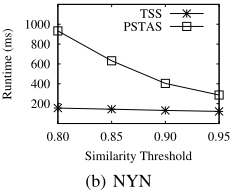
Varying similarity threshold θ. This set of experiments investigates the efficiency as we vary the similarity threshold θ. From Figure 5 we see that the performance of TSS and OriPSTAS is relatively consistent as we vary the value of θ. In contrast, the time cost of PSTAS exhibits a decreasing trend as we increase θ. This can be explained by the effect of our pruning technique. More unqualified trajectory candidates can be pruned when we increase θ, thus the time cost can be reduced substantially.
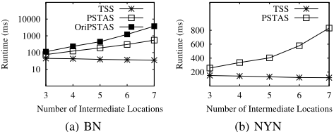
Varying the number of locations |O|. We proceed to study the efficiency of each method as we vary the number of intermediate locations |O|. Figure 6 shows that the time cost of TSS is consistent as we vary |O|. While the time costs of PSTAS and OriPSTAS increase when the number of locations increases. The reason is that a higher value of |O| indicates more partitionings to be evaluated.
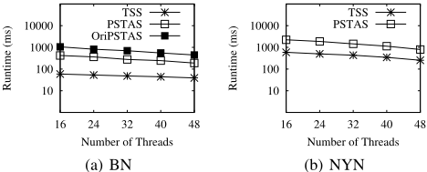
Effect of thread counts. Finally, we study the effect of thread count on the efficiency of all methods. Figure 7 show that all methods exhibit lowered time cost as we increase the number of threads. The results show that all methods are capable of parallel processing.
5 RelatedWork
Trajectory similarity search has been extensively investigated by existing studies. In particular, given a collection of trajectories, the problem of trajectory similarity search aims to find trajectories that meet query arguments defined by users [Frentzos et al., 2007; Zheng et al., 2013; Shang et al., 2012; Driemel et al., 2020; Zheng et al., 2017; Xie et al., 2017; Yuan and Li, 2019; Shang et al., 2014]. The query arguments can be spatial requirement [Chen et al., 2010], temporal requirement [Shang et al., 2014], and textbased requirements [Shang et al., 2012; Zheng et al., 2013]. The problem of trajectory similarity search by multiple locations was first investigated by Chen et al. [Chen et al., 2010]. Specifically, the problem takes a location set from road networks as argument and finds trajectories that are spatially close to the query location set on the basis of some specific metrics. Existing studies on this matter aim to develop spatial and network indexing structures for effectively organizing a large volume of trajectory data [Zheng et al., 2018; Zhao et al., 2018; Liu et al., 2016; Liu et al., 2014; Chen et al., 2020]. However, the aforementioned studies are developed for supporting the retrieval of existing trajectories. They do not consider the problem of deriving new trajectories by splitting and aligning existing trajectories. [Chen et al., 2019] target the problem of route recommendation by combining past travel routes. However, their proposal does not consider the temporal dimension in route combination.
6 Conclusions
We define and study the problem of Sub-Trajectory Alignment (STA), aiming to address the limitation of low result quality for traditional trajectory similarity search with insufficient trajectory data. To solve the STA problem, we develop a PSTAS algorithm consisting of two phases: (1) Generation of trajectory candidates through network expansion and (2) alignment of trajectory candidates through bottom-up merging. The experiment results confirm that: (1) Answering the STA problem is substantially more likely to find high-quality trajectory results in comparison to answering existing trajectory similarity search problem; (2) Our PSTAS algorithm is capable of answering the STA problem over a collection of up to 10M trajectories with user interaction time.
Acknowledgments
This work was supported by the NSFC (U2001212, 62032001, and 61932004).
@inproceedings{ijcai2021p497,
  title     = {Parallel Subtrajectory Alignment over Massive-Scale Trajectory Data},
  author    = {Chen, Lisi and Shang, Shuo and Feng, Shanshan and Kalnis, Panos},
  booktitle = {Proceedings of the Thirtieth International Joint Conference on
               Artificial Intelligence, {IJCAI-21}},
  publisher = {International Joint Conferences on Artificial Intelligence Organization},
  editor    = {Zhi-Hua Zhou},
  pages     = {3613--3619},
  year      = {2021},
  month     = {8},
  note      = {Main Track},
  doi       = {10.24963/ijcai.2021/497},
  url       = {https://doi.org/10.24963/ijcai.2021/497},
}
TY - CPAPER TI - Parallel Subtrajectory Alignment over Massive-Scale Trajectory Data AU - Chen, Lisi AU - Shang, Shuo AU - Feng, Shanshan AU - Kalnis, Panos T2 - Proceedings of the Thirtieth International Joint Conference on Artificial Intelligence, IJCAI-21 PB - International Joint Conferences on Artificial Intelligence Organization PY - 2021 SP - 3613 EP - 3619 DO - 10.24963/ijcai.2021/497 UR - https://doi.org/10.24963/ijcai.2021/497 ER -Copied
Machine-readable versions of this paper, for tools and AI agents:





