
Neural Relation Inference for Multi-dimensional Temporal Point Processes via Message Passing Graph
Proceedings of the Thirtieth International Joint Conference on Artificial Intelligence. Main Track. Pages 3406-3412.
https://doi.org/10.24963/ijcai.2021/469
Keywords
- Machine Learning: Time-series; Data Streams
- Machine Learning: Relational Learning
Abstract
Relation discovery for multi-dimensional temporal point processes (MTPP) has received increasing interest for its importance in prediction and interpretability of the underlying dynamics. Traditional statistical MTPP models like Hawkes Process have difficulty in capturing complex relation due to their limited parametric form of the intensity function. While recent neural-network-based models suffer poor interpretability. In this paper, we propose a neural relation inference model namely TPP-NRI. Given MTPP data, it adopts a variational inference framework to model the posterior relation of MTPP data for probabilistic estimation. Specifically, assuming the prior of the relation is known, the conditional probability of the MTPP conditional on a sampled relation is captured by a message passing graph neural network (GNN) based MTPP model. A variational distribution is introduced to approximate the true posterior. Experiments on synthetic and real-world data show that our model outperforms baseline methods on both inference capability and scalability for high-dimensional data.
- [Achab et al., 2017] Massil Achab, Emmanuel Bacry, Stéphane Gaïffas, Iacopo Mastromatteo, and Jean- Franc ¸ois Muzy. Uncovering causality from multivariate Hawkes integrated cumulants. JMLR, 2017.
- [Alet et al., 2019] Ferran Alet, Erica Weng, Tomás Lozano- Pérez, and Leslie Pack Kaelbling. Neural relational infer- ence with fast modular meta-learning. In NeurIPS, 2019.
- [Chung et al., 2014] Junyoung Chung, Caglar Gulcehre, KyungHyun Cho, and Yoshua Bengio. Empirical evalua- tion of gated recurrent neural networks on sequence mod- eling. In NIPS Workshop on Deep Learning, 2014.
- [Daley and David, 2007] D.J. Daley and Vere-Jones David. An Introduction to the Theory of Point Processes: Vol- ume II: General Theory and Structure. Springer Science & Business Media, 2007.
- [Du et al., 2016] Nan Du, Hanjun Dai, Rakshit Trivedi, Utkarsh Upadhyay, Manuel Gomez-Rodriguez, and Le Song. Recurrent marked temporal point processes: Em- bedding event history to vector. In KDD, 2016.
- [Eichler et al., 2017] Michael Eichler, Rainer Dahlhaus, and Johannes Dueck. Graphical modeling for multivari- ate Hawkes processes with nonparametric link functions. Journal of Time Series Analysis, 2017.
- [Etesami et al., 2016] Jalal Etesami, Negar Kiyavash, Kun Zhang, and Kushagra Singhal. Learning network of multi- variate Hawkes processes: A time series approach. In UAI, 2016.
- [Graber and Schwing, 2020] Colin Graber and Alexander Schwing. Dynamic neural relational inference. In CVPR, 2020.
- [Hoffman et al., 2013] Matthew D. Hoffman, David M. Blei, Wang Chong, and John Paisley. Stochastic variational in- ference. JMLR, 14, 2013.
- [Jain and Wallace, 2019] Sarthak Jain and Byron C Wallace. Attention is not explanation. In NAACL-HLT, 2019.
- [Jia and Benson, 2019] Junteng Jia and Austin R. Benson. Neural jump stochastic differential equations. In NeurIPS, 2019.
- [Kipf et al., 2018] Thomas Kipf, Ethan Fetaya, Kuan-Chieh Wang, Max Welling, and Richard Zemel. Neural relational inference for interacting systems. In ICML, 2018.
- [Li et al., 2018] Shuang Li, Shuai Xiao, Shixiang Zhu, Nan Du, Yao Xie, and Le Song. Learning temporal point pro- cesses via reinforcement learning. In NeurIPS, 2018.
- [Linderman and Adams, 2014] Scott W. Linderman and Ryan P. Adams. Discovering latent network structure in point process data. In ICML, 2014.
- [Liu et al., 2018] Yanchi Liu, Tan Yan, and Haifeng Chen. Exploiting graph regularized multi-dimensional Hawkes processes for modeling events with spatio-temporal char- acteristics. In IJCAI, 2018. IJCAI
- [Paranjape et al., 2017] Ashwin Paranjape, Austin R. Ben- son, and Jure Leskovec. Motifs in temporal networks. In WSDM, 2017.
- [Salehi et al., 2019] Farnood Salehi, William Trouleau, Matthias Grossglauser, and Patrick Thiran. Learning Hawkes processes from a handful of events. In NeurIPS, 2019.
- [Shang and Sun, 2019] Jin Shang and Mingxuan Sun. Geo- metric Hawkes processes with graph convolutional recur- rent neural networks. In AAAI, 2019.
- [Trivedi et al., 2019] Rakshit Trivedi, Mehrdad Farajtabar, Prasenjeet Biswal, and Hongyuan Zha. Dyrep: Learning representations over dynamic graphs. In ICML, 2019.
- [Wang et al., 2017] Yongqing Wang, Huawei Shen, Shenghua Liu, Jinhua Gao, and Xueqi Cheng. Cas- cade dynamics modeling with attention-based recurrent neural network. In IJCAI, 2017. IJCAI
- [Webb et al., 2019] Ezra Webb, Ben Day, Helena Andres- Terre, and Pietro Lió. Factorised neural relational infer- ence for multi-interaction systems. In ICML Workshop on Learning and Reasoning with Graph-Structured Data, 2019.
- [Wiegreffe and Pinter, 2019] Sarah Wiegreffe and Yuval Pin- ter. Attention is not not explanation. In EMNLP-IJCNLP, 2019.
- [Wu et al., 2019] Qitian Wu, Zixuan Zhang, Xiaofeng Gao, Junchi Yan, and Guihai Chen. Learning latent process from high-dimensional event sequences via efficient sam- pling. In NeurIPS, 2019.
- [Wu et al., 2020] Weichang Wu, Huanxi Liu, Xiaohu Zhang, Yu Liu, and Hongyuan Zha. Modeling event propagation via graph biased temporal point process. IEEE TNNLS, 2020.
- [Xiao et al., 2017] Shuai Xiao, Mehrdad Farajtabar, Xiao- jing Ye, Junchi Yan, Le Song, and Hongyuan Zha. Wasser- stein learning of deep generative point process models. In NIPS, 2017.
- [Xiao et al., 2019] Shuai Xiao, Junchi Yan, Mehrdad Fara- jtabar, Le Song, Xiaokang Yang, and Hongyuan Zha. Learning time series associated event sequences with re- current point process networks. IEEE TNNLS, 2019.
- [Zhang et al., 2019] Cheng Zhang, Judith Bütepage, Hedvig Kjellström, and Stephan Mandt. Advances in variational inference. IEEE TPAMI, 2019.
- [Zhou et al., 2013a] Ke Zhou, Hongyuan Zha, and Le Song. Learning social infectivity in sparse low-rank networks us- ing multi-dimensional Hawkes processes. In AISTATS, 2013.
- [Zhou et al., 2013b] Ke Zhou, Hongyuan Zha, and Le Song. Learning triggering kernels for multi-dimensional Hawkes processes. In ICML, 2013.
- [Zuo et al., 2018] Yuan Zuo, Guannan Liu, Hao Lin, Jia Guo, Xiaoqian Hu, and Junjie Wu. Embedding temporal network via neighborhood formation. In KDD, 2018.
References were extracted automatically from the PDF and may contain errors.
Full text extracted automatically from the PDF; figures, tables and equations may differ. The PDF is the version of record.
1 Introduction
Many real-world temporal processes involving time-stamped multi-typed event sequences can be modeled by Multivariate or namely Multi-dimensional Temporal Point Processes (MTPP) [Daley and David, 2007], e.g. earthquake records, stock transactions and information spread on social networks. Entities along each dimension in MTPP may have complex relations among multiple dimensions. For instance, in online social networks, multiple users' behavior sequences form an MTPP. "Friendship" relationships among users form a latent relation graph. Information spreading via graph edges can affect users' behaviors (MTPP). Knowing relationships among dimensions is of great interest to multiple parties.
However, in real-world scenarios, the relation is often implicit and calls for effective inference. Many relation inference methods for MTPP [Zhou et al., 2013a; Linderman and Adams, 2014; Eichler et al., 2017; Liu et al., 2018] resort to the so-called Multivariate Hawkes Processes (MHP) . However, MHP makes strong assumption about the underlying dynamics of MTPP. Thus, it is hard for these MHP-baesd models to capture complex real-world dynamics.
∗Corresponding author is Junchi Yan.
Meanwhile, MTPP can be modeled by Recurrent Neural Networks [Du et al., 2016], Generative Adversarial Networks [Xiao et al., 2017], Reinforcement Learning [Li et al., 2018; Wu et al., 2019] and Neural Ordinary Differential Equation [Jia and Benson, 2019]. Yet these neural-networkbased models mainly focus on probability modeling and event prediction, instead of relation inference. The attention model in [Xiao et al., 2019; Wang et al., 2017] may be used to infer the relation, while the interpretability is still controversial [Jain and Wallace, 2019; Wiegreffe and Pinter, 2019].
To fill the gap, we propose Neural Relation Inference for Multi-dimensional Temporal Point Processes (TPP-NRI). We use a variational inference framework which allows us to incorporate prior knowledge about the relation. We assume the prior of the relation is known. A neural model based on message passing graph is used to estimate conditional probability of an MTPP conditional on a sampled relation matrix. Our goal is to estimate the posterior of the relation. Thus a variational distribution is introduced to approximate the true posterior. The contributions of our work are as follows.
i) We develop a message passing graph model for multidimensional temporal point processes. Our model can model more complex dynamics than traditional statistical models and enjoys a clear probabilistic meaning in contrast to the few existing neural-network-based works [Xiao et al., 2019; Wang et al., 2017] which resort to attention mechanisms.
ii) We propose a variational inference framework for neural MTPP relation inference. The framework can incorporate different relation priors, thanks to its probabilistic nature. To our best knowledge, this is the first work for probabilistic relation discovery for MTPP using deep neural networks.
iii) Experimental results on both synthetic and real-world benchmarks show the effectiveness of our approach, for both model fitting as well as scalability for high-dimensional data.
2 Preliminaries and RelatedWorks
2.1 Multi-dimensional Temporal Point Process
MTPP [Daley and David, 2007] is a useful tool to model a group of correlated processes in continuous-time domain. For a D-dimensional TPP, we use Ni(t), i = 1, . . . , D, t ∈ [0, T ) to denote the counting process which counts the number of events in dimension i until time t. An MTPP can be modeled by its conditional intensity function:
where Ht denotes the historical observations until t.
We denote a sequence of events as S = {(tn, in)}Nn=1 , where tn ∈ [0, T) is the timestamp of n-th event and in ∈ {1, . . . ,D} is the dimension. The log likelihood of S is:
Traditional statistical MTPP models design different parametric forms, e.g. Hawkes process for the conditional intensity function, to capture underlying dynamics of various processes. Maximum Likelihood Estimation (MLE) is used to estimate parameters in the models by optimizing Eq. 2.
2.2 Traditional Relation Inference for MTPP
As a popular MTPP model, a typical embodiment of Multivariate Hawkes Process (MHP) defines the intensity as:
where µj ≥ 0 is the base intensity and g(t) ≥ 0 is the kernel function representing the influence of an event. W ∈ RD×D ≥0 is called infectivity matrix which captures the exciting relation: larger Wji means that an event of dimension i is more likely to trigger events of j. Most works on MTPP relation inference focus on learning the infectivity matrix.
For MHP, it has been show in [Eichler et al., 2017] that whether events in dimension i Granger-causes events in j equals to if Wji = 0. [Etesami et al., 2016] proves that the infectivity matrix is equivalent to the Directed Information graph (DIGs). [Zhou et al., 2013a] adds nuclear norm and ℓ1 norm to the objective to enforce the learned matrix to be sparse and low-rank, and uses alternating direction method of multipliers and majorization minimization (ADM4) to solve the optimization problem. [Linderman and Adams, 2014] adds a binary mask to the infectivity matrix to control whether Wji = 0. [Salehi et al., 2019] devises a variational model with tunable hyper-parameters of regularization. [Liu et al., 2018] uses external spatio information for regularization.
However, these methods are based on MHP, which makes strong parametric assumption. It is hard for MHP to capture complex relations. Nonparametric methods [Zhou et al., 2013b; Achab et al., 2017] are also proposed, but their generalization ability are still limited with a shallow model.
2.3 Neural Relation Inference for Time-series
Different from MTPP data where events happen irregularly, time-series (TS) is synchronous and regularly-sampled. As time-series is measured at grid points, it is easier to model it using neural networks, as well as for relation inference.
The work [Kipf et al., 2018] introduces an unsupervised model called Neural Relation Inference (NRI) to infer relation from time-series data. NRI uses a variational autoencoder (VAE) framework where the encoder and decoder are modeled by graph neural networks (GNN). [Webb et al., 2019] expands NRI by representing relation with a multiplex graph and proposes Factorised Neural Relational Inference (fNRI). [Graber and Schwing, 2020] thinks that the relation changes as time progresses and develops Dynamic Neural Relational Inference (dNRI). [Alet et al., 2019] uses a metalearning framework to solve the relation inference problem so that relations among dimensions can be dependent.
| Methods | Data | Model | Prob. Relation |
|---|---|---|---|
| [Zhou et al., 2013a] [Linderman and Adams, [Liu et al., 2018] [Salehi et al., 2019] [Kipf et al., 2018] [Webb et al., 2019] [Alet et al., 2019] [Graber and Schwing, 2020] [Wang et al., 2017] [Xiao et al., 2019] | MTPP MTPP MTPP TS TS TS TS | MHP MHP MHP MHP | 7 7 7 7 7 |
| 2014] | |||
| MTPP | |||
| 3 | |||
| Neural | 3 | ||
| Neural | 3 | ||
| Neural | 3 | ||
| Neural | 3 | ||
| MTPP | Neural | ||
| MTPP | Neural | ||
| TPP-NRI (Ours) | MTPP | Neural | 3 |
These neural-network-based models all focus on TS data, which cannot be applied to MTPP data, as the latter is irregular, asynchronous and more sparse in time domain.
Further Remarks. Note the neural network models [Xiao et al., 2019; Wang et al., 2017] also mention using attention for relation inference, though the main purpose of their methods are event prediction. Attention's physical meaning is still not fully clear [Jain and Wallace, 2019; Wiegreffe and Pinter, 2019]. Differently, our model provides probability estimation of the relation, which is more interpretable. Table 1 compares our work to peer methods. Our neural method has higher capacity than traditional parametric models, while in the meanwhile it has more rigorous probabilistic meaning than existing neural models. To our best knowledge, this is the first work for neural probabilistic relation mining for MTPP data.
3 Neural Relation Inference for MTPP
In Section 3.1, we first formulate the problem for relation inference, and then provide a variational inference framework in Section 3.2. The framework involves a probability term estimated by the MTPP model in Section 3.3. The whole model is efficiently trained in Section 3.4.
3.1 Problem Setting and Formulation
Given observed multivariate event sequences, our goal is to infer whether there exists interaction over dimensions. Consider we have M samples of D-dimensional TPP with observations S = {Sm}Mm=1 , where Sm = {(tmn , imn )}Nm n=1 , tmn ∈ [0, T), imn ∈ {1, . . . ,D}. We assume these sequences are generated by the same latent dynamic. Our goal is to infer a binary adjacency matrix A ∈ {0, 1}D×D for the underlying relation among dimensions: Aji = 1 iff occurrence of events in dimension i affects that of j.
Note that like many neural relation inference models [Kipf et al., 2018; Alet et al., 2019; Webb et al., 2019; Graber and Schwing, 2020], our model signifies if there is an interaction, but not the exact description (e.g. excitation or inhibition or other more dynamic influences). In contrast, MHP models' interaction has a clear meaning but is limited to excitation.
3.2 Model Framework and Overall Objective
We take a relation matrix estimation perspective to the inference task. Given event sequences S, we assume these sequences share the same latent relation matrix A. Rather than just giving a deterministic binary estimation like [Linderman and Adams, 2014], we provide a probabilistic framework.
Given prior p(A), we use an MTPP model (detailed in Section 3.3) to model the conditional pθ(S|A). The goal is to maximum the marginal distribution pθ(S), then get the posterior pθ(A|S). As the true posterior has no analytical solution, we use Variational Inference (VI) [Zhang et al., 2019] for approximation. A global variational distribution qφ(A) parameterized by φ is used to approximate pθ(A|S). We need to minimize the KL divergence between qφ(A) and pθ(A|S):
Rearrange the above formula, we can get:
Maximizing the defined L(θ, φ; S) in Eq. 4 is equivalent to minimizing KL divergence and maximizing log pθ(S). Then, the problem changes to maximize L(θ, φ; S), which is called the evidence lower bound (ELBO) [Hoffman et al., 2013]:
Assume that p(A) is a discrete probability distribution where p(A) = ∏j̸=i p(Aji = 1) and so is qφ. Then the first term in Eq. 6 can be computed by (cross) entropy:
Specific prior can be introduced based on domain knowledge: e.g. setting p(Aji = 1) = 0.2 encourages the learned posterior to be sparse.
As the second term in Eq. 6 is intractable, we approximate it through sampling. Sampling a relation A, the task becomes to model the conditional probability pθ(S|A).
3.3 Conditional ProbabilityModeling viaMessage Passing Graph Based MTPP model
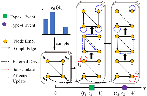
Sampling a relation matrix A, we propose a model based on message passing Graph Neural Network (GNN) and RNN to model the conditional probability, as sketched in Figure 1.
For D-dimensional TPPs, we use hi(t) ∈ Rd to represent hidden state of dimension i at time t. Thus at time t ∈ [0, T), we have a set of vectors H(t) = {hi(t)}Di=1 . A can be viewed as the adjacency matrix of a directed graph and H(t) can be viewed as the embedding vectors of D nodes. This forms a directed unweighted graph G = {H(t),A}. Every time an event (tn, in) occurs, H(t) will be updated by three processes: External Drive, Self-Update and Affected-Update.
1) External Drive. MTPP can be affected by some external forces. Thus the node representation can change smoothly even no event occurs. We use External Drive process to model the smooth update between two consecutive events:
where ∆tn = tn - tn-1 is the time interval of two events. The selected function fExt should satisfy two conditions:
- fExt(h, 0) = h
For computational efficiency, we simply set:
2) Self-Update. The occurrence of an event in dimension in will change state of node in. Because the update should be related to its previous state, we use RNN for Self-Update:
We use Gated Recurrent Unit (GRU) [Chung et al., 2014] for update. Note Self-Update only updates the latent state of dimension in, which is the dimension of occurred event. States of other dimensions hj(t-n ), ∀j ̸= in remain unchanged.
3) Affected-Update. Event in dimension in can also affect the hidden states of other dimensions j ̸= in. We think that this influence should relate to both hin and h-j . We use message passing to model this process:
The first equation in Eq. 11 computes the message passing from node in to node j. fMSG, modeled by a small neural network, computes the original message. And [·, ·] denotes the concatenation operation. Note that in most cases fMSG is asymmetric, which means the message passing from i to j is different from j to i. Recall that Ajin is a binary value to control message passing. If Ajin = 1, the original message is passed to node j; otherwise, a zero vector 0 will be passed.
The second equation in Eq. 11 represents the update process for hj , ∀j ̸= in. Taking the message MSG(in,j)(tn) and the previous state hj(t-n ), we use another GRU for update. A zero vector 0 contains no information about which event occurs, thus the update depends only on the previous state. If the received message is not 0, the update depends on both effect from in (embedded in message) and previous state.
For D-dimensional sequence Sm = {(tn, in)}Nm n=1 , we update the node hidden states using three processes one after another, resulting in a set of hidden vectors at different time points H = {H(ti)}Nm i=1 , where H(ti) ∈ RD×d . Note that hj(t-n ) are just temporary variables which will not be used in the following computation. We now use H to model the conditional intensity. Following [Du et al., 2016], we formulate the intensity of each dimension i by:
where tn < t ≤ tn+1. v is a shared column vector for all dimensions, and wi, bi are unique scalars for each dimension.
Given the above conditional intensity, we can use Eq. 2 to compute the log likelihood of a sequence: log pθ(Sm|A). For a set of sequences S = {Sm}Mm=1 , assuming they are (conditional) independent, one can sum the results up to obtain:
log pθ (S|A)
3.4 Training
Our goal is to get the posterior qφ(A) by optimizing Eq. 6. It is straightforward to compute L and use gradient descent to optimize. However, the expectation of log pθ(S|A) has no analytical solution, we approximate it through sampling. We use Gumbel-Softmax sampling [?] which approximates discrete distributions with continuous ones to provide differentiable samples. Mini-batch gradient descent is also used during training. The overall training process is shown in Algorithm 1. Note that the prior p(A) is fixed.
Remarks. Some works also combine graph structure with MTPP. [Shang and Sun, 2019; Wu et al., 2020; Liu et al., 2018] use some explicit graph structures to improve event prediction accuracy. [Zuo et al., 2018; Trivedi et al., 2019] use MTPP to model topological evolution of dynamic graphs. These methods are orthogonal to ours.
4 Experiments
We implement our model using PyTorch. We set hidden size of GRUSelf and GRUAffect to be 20. fExt is implemented
Algorithm 1 Variational training algorithm for TPP-NRI
Input: Observed sequences S = {Sm}Mm=1 . Sample size L. Prior p(A). Mini-batch size B. Training epochs K. Initial qφ(A) and message passing graph pθ(S|A).
Output: Approximated posterior of (i.e. inferred) relation matrix qφ(A).
- 1: for epcoh ← 1, · · · ,K do
- 2: for iter ← 1, · · · , ⌈ MB ⌉ do
- 3: Sample a batch of sequences S′ from S; //Approximate the 2nd term in ELBO (Eq. 6) by first sampling A then computing conditional likelihood.
- 4: Sample relation matrix A1, · · · ,AL ∼ qφ(A);
- 5: Compute conditional log likelihood log pθ(S′ |Al)
//Compute and optimize the approximated ELBO
- using Eq. 8 to 13. (Eq. 6) by min-batch gradient descent.
- 6: L←Eqφ [log p(A) qφ(A) ] + M BL ∑Ll=1 log pθ(S′ |Al);
- 7: g ← -∇θ,φL;
- 8: θ, φ ← Update parameters using gradient descent.
- 9: end for
- 10: end for
11: return qφ(A).
by a one-layer fully-connected network. Mini-batch size B is set to 32 and sample size L is set to 1. Adam algorithm with learning rate 0.005 is used for optimization.
Following [Linderman and Adams, 2014; Salehi et al., 2019] we perform two tasks: a) link prediction to infer if interactions exist between 2 dimensions, i.e. whether Aji = 1 or not. b) event prediction measuring the probability of next event given past events. Note that it is impossible to estimate the performance of link prediction on real-world data as the ground truth relation is inaccessible. Therefore, we use event prediction task to estimate indirectly.
4.1 Experiments on Synthetic Data
We use a 100-dimensional Hawkes process for data generation. Following [Zhou et al., 2013a], we set the true infecticity W = UV⊤, where U is a 100 × 9 matrix with U10(i-1)+1:10(i+1),i ∼ Uniform(0.1, 0.2), i = 1, . . . , 9, so is V. Then the spectral radius of W is scaled to 0.8. Baseline intensities are set as µi ∼ Uniform(0, 0.02), i = 1, . . . , 100. We use W and µ to generate the following three datasets.
MHP (Exp). MHP with exponential kernels: set kernel function in Eq. 3 as g(t) = β exp (-βt). We set β = 2.5 and T = 20. 2,500 samples are generated from this process. In total, we have 220,235 events in this dataset.
MHP (Power). MHP with power law kernels: set kernel function as g(t) = (δ + t)-β . We set δ = 0.8, β = 2.5 and T = 20. 2,500 samples are generated from this process. In total, we have 155,825 events in this dataset.
MHP (Exp+Power). MHP (Exp) and MHP (Power) are mixed to get a dataset with 5,000 sequences and 376,040 events. As MHP (Exp) and MHP (Power) are generated by the sameW, they share the same latent relation structure.
To mimic real-world data, we add random noises following standard Gaussian distribution to every timestamp. All timestamps are scaled to [0, 1] for model input. For each dataset, we randomly sample 80% for training and 20% for testing.
Following [Linderman and Adams, 2014; Salehi et al., 2019], we use the following three metrics (the first two are for link prediction, the third is for event prediction):
F1-score. Considering that not all outputs have clear physical meaning like ours, we threshold at 10-quantiles between the min and max value of output matrices and compute the corresponding F1-scores. The best result out of 10 is selected. Following [Zhou et al., 2013a], we only consider Aji, j ̸= i.
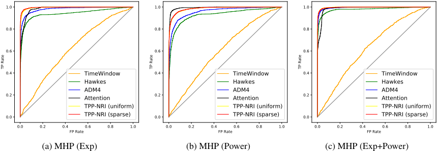
ROCcurve. We threshold at every point of the inferredmatrix and plot Receiver Operating Characteristic Curve (ROC).
Log Likelihood (LL). We estimate LL (Eq. 13) on test set. For presentation, we normalize LL by number of events.
We compare the performance of the following models:
- TimeWindow. Divide [0, T) into bins with equal length. For each dimension, number of events in each bin is counted. The cosine similarity of vectors is used as relation matrix.
- Hawkes. Hawkes process with exponential kernels.
- ADM4. Alternating direction method of multipliers and majorization minimization for Hawkes process with sparse and low-rank regularization [Zhou et al., 2013a].
- Attention. RNN model with attention mechanism similar to [Xiao et al., 2019; Wang et al., 2017]. Average attention matrix among all event sequences is used as inferred relation.
- TPP-NRI (uniform). Our neural relation model without prior knowledge (by setting p(Aji = 1) = 0.5).
- TPP-NRI (sparse). Our neural relation model with prior that the relation is sparse (by setting p(Aji = 1) = 0.2).
- TPP-NRI (full). Fix the graph as complete graph and use
- the proposed message passing graph to model log likelihood.
- TPP-NRI (true). Input the real graph structure into the message passing graph to model log likelihood.
TimeWindow is only for F1-score and ROC curve estimation, TPP-NRI (full and true) are only for LL estimation. For TPP-NRI (uniform and sparse), we sample 100 graphs from posterior qφ(A) and estimate the mean LL.
Results. ROC curves are shown in Figure 2, F1-score and LL are given in Table 2. As for link prediction, ROC curves and F1-score show that our two TPP-NRI (uniform and sparse) outperform traditional methods (Timewindow, Hawkes and ADM4) on all datasets. Sparse prior can slightly improve the performance. Attention performs better on MHP (Power), but is not as interpretable as TPP-NRI: output of TPP-NRI has clear meaning: probability of interaction.
As for LL estimation, TPP-NRI (true) significantly outperforms all other methods. This shows that knowing the relation is of great help in event prediction and emphasizes the importance of relation inference. TPP-NRI (full) performs well, but it can not perform relation inference. For relation inference methods, TPP-NRI models outperform baseline models on MHP (Exp) and MHP (Exp+Power), but are outperformed by ADM4 on MHP (Power). However, the gap is small and our models are more interpretable according to link prediction.
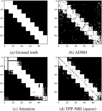
We further show the inferred relation on MHP (Exp) dataset in Figure 3. It is easy to see that matrix inferred by TPP-NRI has less false negative (near the diagonal) and false positive (around corners) points than ADM4. Attention tends to output more edges than ground truth relation.
| Methods | MHP (Exp) | MHP (Power) | MHP (Exp+Power) |
|---|---|---|---|
| TimeWindow | .457/∞ | .448/∞ | .466/∞ |
| Hawkes | .842/-.743 | .805/-1.26 | .910/-.950 |
| ADM4 | .897/-.715 | .839/-1.24 | .941/-.958 |
| Attention | .881/-.767 | .934/-1.27 | .914/-.966 |
| TPP-NRI (uniform) | .941/-.711 | .898/-1.25 | .959/-.916 |
| TPP-NRI (sparse) | .954/-.699 | .904/-1.25 | .958/-.918 |
| TPP-NRI (full) | ∞/-.661 | ∞/-1.23 | ∞/-.892 |
| TPP-NRI (true) | ∞/-.654 | ∞/-1.22 | ∞/-.886 |
| Methods | Stack Overflow | Stock | |
|---|---|---|---|
| Hawkes | 0.272 | -0.834 | -1.22 |
| ADM4 | 0.306 | 0.107 | -1.69 |
| Attention | 0.367 | 1.13 | 1.16 |
| TPP-NRI (uniform) | 0.370 | 1.83 | 1.30 |
| TPP-NRI (sparse) | 0.378 | 1.76 | 1.33 |
| TPP-NRI (full) | 0.480 | 2.02 | 1.32 |
4.2 Experiments on Real-world Data
We also evaluate performance on three real-world datasets:
Stack Overflow contains question answering records on Stack Overflow over 2,774 days [Paranjape et al., 2017]. Every time a user answers a question is recorded as an event with the user ID as the dimension. We consider the most active 100 users which correspond to 783,085 events. We use events in every half day as a sample of sequence.
Email contains email sending records of 142 members in a large European research institution during 803 days [Paranjape et al., 2017]. Every time a member sends an email is recorded as an event with the sender's ID as the dimension. In total, we have 48,141 events in this dataset. Events in every 24 hours are viewed as a sample of sequence.
Stock contains daily stock prices of 31 companies(www.kaggle.comszrleestock-time-series-20050101to-20171231). A stock changes by ±1% of last day's price is recorded as an event with the ID as the dimension [Salehi et al., 2019]. This dataset contains 36,356 events. Events of a
month are viewed as a sample of sequence.
All timestamps are scaled to [0, 1]. For each dataset, we randomly sample 80% for training and the rest for testing.
For TPP-NRI, we use same prior as synthetic experiments. Table 3 shows that our models significantly outperform baselines. TPP-NRI (sparse) even outperforms TPP-NRI (full) on Stock, although its main task is relation inference.
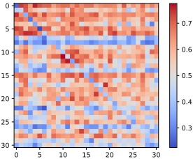
Figure 4 shows the relation of Stock inferred by TPPNRI (sparse). Stock 0 ∼ 6 are information technology companies, which are likely to be affected by others and have stronger interaction within the group. Stock 17 and 19 have high probability to interact each other. Actually, they are Chevron Corporation and Exxon Mobil Corporation which are the only two petroleum industry companies. This shows that our model really uncovers useful information.
4.3 Scalability for High-dimensional Data
We use process similar to Sec. 4.1 to generate MHP (Exp) data of different dimensions and test the scalability. We estimate the overall training time (in second) and the epochs for convergence (maximum value is set 50). TPP-NRI runs on a single RTX-2080Ti (11GB) GPU and ADM4 runs on a core of Intel i9-7920X CPU @ 2.90GHz with 128GB RAM, as ADM4 involves CPU-intensive computing. Table 4 shows that our model outperforms ADM4. The gap gets greater as the dimension increases. This is because the use of neural network, which not only captures complex dynamics but also enjoys acceleration by parallel computing architectures.
| dim | F1-score | Overall training time (epoch) | ||
|---|---|---|---|---|
| ADM4 | TPP-NRI | ADM4 | TPP-NRI | |
| 100 | 0.957 | 0.960 | 3,799(44) | 932(10) |
| 200 | 0.813 | 0.898 | 10,380(50) | 2,024(14) |
| 300 | 0.713 | 0.843 | 16,947(50) | 2,930(14) |
| 400 | 0.584 | 0.783 | 26,195(50) | 4,092(18) |
| 500 | 0.452 | 0.720 | 34,418(50) | 3,672(14) |
5 Conclusion
This paper aims to infer the underlying relation among dimensions for a temporal point process, which is fulfilled by message passing on relation graph via variational learning. Our method enjoys more rigorous probabilistic formulation and physical meaning than those attention based models and it also outperforms traditional parametric models.
Acknowledgements
This work was partly supported by National Key Research and Development Program of China (2020AAA0107600), NSFC (61972250, 72061127003), and Shanghai Municipal Science and Technology Major Project (2021SHZDZX0102).
@inproceedings{ijcai2021p469,
  title     = {Neural Relation Inference for Multi-dimensional Temporal Point Processes via Message Passing Graph},
  author    = {Zhang, Yunhao and Yan, Junchi},
  booktitle = {Proceedings of the Thirtieth International Joint Conference on
               Artificial Intelligence, {IJCAI-21}},
  publisher = {International Joint Conferences on Artificial Intelligence Organization},
  editor    = {Zhi-Hua Zhou},
  pages     = {3406--3412},
  year      = {2021},
  month     = {8},
  note      = {Main Track},
  doi       = {10.24963/ijcai.2021/469},
  url       = {https://doi.org/10.24963/ijcai.2021/469},
}
TY - CPAPER TI - Neural Relation Inference for Multi-dimensional Temporal Point Processes via Message Passing Graph AU - Zhang, Yunhao AU - Yan, Junchi T2 - Proceedings of the Thirtieth International Joint Conference on Artificial Intelligence, IJCAI-21 PB - International Joint Conferences on Artificial Intelligence Organization PY - 2021 SP - 3406 EP - 3412 DO - 10.24963/ijcai.2021/469 UR - https://doi.org/10.24963/ijcai.2021/469 ER -Copied
Machine-readable versions of this paper, for tools and AI agents:





