
Exploiting Graph Regularized Multi-dimensional Hawkes Processes for Modeling Events with Spatio-temporal Characteristics
Proceedings of the Twenty-Seventh International Joint Conference on Artificial Intelligence. Main track. Pages 2475-2482.
https://doi.org/10.24963/ijcai.2018/343
Keywords
- Machine Learning: Time-series;Data Streams
- Machine Learning Applications: Applications of Unsupervised Learning
Abstract
Multi-dimensional Hawkes processes (MHP) has been widely used for modeling temporal events. However, when MHP was used for modeling events with spatio-temporal characteristics, the spatial information was often ignored despite its importance. In this paper, we introduce a framework to exploit MHP for modeling spatio-temporal events by considering both temporal and spatial information. Specifically, we design a graph regularization method to effectively integrate the prior spatial structure into MHP for learning influence matrix between different locations. Indeed, the prior spatial structure can be first represented as a connection graph. Then, a multi-view method is utilized for the alignment of the prior connection graph and influence matrix while preserving the sparsity and low-rank properties of the kernel matrix. Moreover, we develop an optimization scheme using an alternating direction method of multipliers to solve the resulting optimization problem. Finally, the experimental results show that we are able to learn the interaction patterns between different geographical areas more effectively with prior connection graph introduced for regularization.
- [Boyd et al., 2011] S. Boyd, N. Parikh, E. Chu, B. Peleato, and J. Eckstein. Distributed optimization and statistical learning via the alternating direction method of multiplier- s. Foundations and Trends R in Machine Learning, 2011.
- [Cai et al., 2011] Deng Cai, Xiaofei He, Jiawei Han, and Thomas S Huang. Graph regularized nonnegative ma- trix factorization for data representation. IEEE Trans- actions on Pattern Analysis and Machine Intelligence, 33(8):1548-1560, 2011.
- [Embrechts et al., 2011] Paul Embrechts, Thomas Liniger, and Lu Lin. Multivariate hawkes processes: an appli- cation to financial data. Journal of Applied Probability, 48(A):367-378, 2011.
- [Kamarianakis et al., 2012] Yiannis Kamarianakis, Wei Shen, and Laura Wynter. Real-time road traffic fore- casting using regime-switching space-time models and adaptive lasso. Applied stochastic models in business and industry, 28(4):297-315, 2012.
- [Li and Zha, 2016] Liangda Li and Hongyuan Zha. House- hold structure analysis via hawkes processes for enhancing energy disaggregation. In IJCAI, pages 2553-2559, 2016. IJCAI
- [Li et al., 2014] Liangda Li, Hongbo Deng, Anlei Dong, Y- i Chang, and Hongyuan Zha. Identifying and labeling search tasks via query-based hawkes processes. In Pro- ceedings of the 20th ACM SIGKDD international con- ference on Knowledge discovery and data mining, pages 731-740. ACM, 2014.
- [Lippi et al., 2013] Marco Lippi, Matteo Bertini, and Paolo Frasconi. Short-term traffic flow forecasting: An experi- mental comparison of time-series analysis and supervised learning. IEEE Transactions on Intelligent Transportation Systems, 14(2):871-882, 2013.
- [Liu et al., 2014] Qi Liu, Enhong Chen, Hui Xiong, Yong Ge, Zhongmou Li, and Xiang Wu. A cocktail approach for travel package recommendation. IEEE Transactions on Knowledge and Data Engineering, 26(2):278-293, 2014.
- [Liu et al., 2015] Bin Liu, Hui Xiong, Spiros Papadimitriou, Yanjie Fu, and Zijun Yao. A general geographical proba- bilistic factor model for point of interest recommendation. IEEE Transactions on Knowledge and Data Engineering, 27(5):1167-1179, 2015.
- [Liu et al., 2016] Yanchi Liu, Chuanren Liu, Bin Liu, Meng Qu, and Hui Xiong. Unified point-of-interest recommen- dation with temporal interval assessment. In Proceedings of KDD, pages 1015-1024. ACM, 2016.
- [Liu et al., 2017] Yanchi Liu, Chuanren Liu, Xinjiang Lu, Mingfei Teng, Hengshu Zhu, and Hui Xiong. Point-of- interest demand modeling with human mobility pattern- s. In Proceedings of the 23rd ACM SIGKDD Internation- al Conference on Knowledge Discovery and Data Mining, pages 947-955. ACM, 2017.
- [Marsan and Lengline, 2008] David Marsan and Olivier Lengline. Extending earthquakes' reach through cascad- ing. Science, 319(5866):1076-1079, 2008.
- [Tobler, 1970] Waldo R Tobler. A computer movie simulat- ing urban growth in the detroit region. Economic geogra- phy, 46(sup1):234-240, 1970.
- [Wang et al., 2017] Pengfei Wang, Yanjie Fu, Guannan Li- u, Wenqing Hu, and Charu Aggarwal. Human mobility synchronization and trip purpose detection with mixture of hawkes processes. In Proceedings of the 23rd ACM SIGKDD International Conference on Knowledge Discov- ery and Data Mining, pages 495-503. ACM, 2017.
- [Xu et al., 2013] Chang Xu, Dacheng Tao, and Chao Xu. A survey on multi-view learning. arXiv preprint arX- iv:1304.5634, 2013.
- [Xu et al., 2017] Hongteng Xu, Weichang Wu, Shamim Ne- mati, and Hongyuan Zha. Patient flow prediction via discriminative learning of mutually-correcting processes. IEEE transactions on Knowledge and Data Engineering, 29(1):157-171, 2017.
- [Yang and Zha, 2013] Shuang-Hong Yang and Hongyuan Zha. Mixture of mutually exciting processes for viral dif- fusion. In International Conference on Machine Learning, pages 1-9, 2013.
- [Ye et al., 2011] Mao Ye, Peifeng Yin, Wang-Chien Lee, and Dik-Lun Lee. Exploiting geographical influence for col- laborative point-of-interest recommendation. In Proceed- ings of the 34th international ACM SIGIR conference on Research and development in Information Retrieval, pages 325-334. ACM, 2011.
- [Zhang et al., 2017] Junbo Zhang, Yu Zheng, and Dekang Qi. Deep spatio-temporal residual networks for citywide crowd flows prediction. In AAAI, pages 1655-1661, 2017.
- [Zhou et al., 2013] Ke Zhou, Hongyuan Zha, and Le Song. Learning social infectivity in sparse low-rank networks us- ing multi-dimensional hawkes processes. In Artificial In- telligence and Statistics, pages 641-649, 2013.
References were extracted automatically from the PDF and may contain errors.
Full text extracted automatically from the PDF; figures, tables and equations may differ. The PDF is the version of record.
1 Introduction
Large-scale spatio-temporal data have been accumulated in various applications, such as criminal records frommunicipal systems and bike rental transactions from bike sharing systems. These fine-grained data can naturally be regarded as sequences of events over different locations, where each event may trigger or influence a series of subsequent events under certain intrinsic spatial structure due to their geographical proximity. For example, a pickpocket may attempt to replicate a previous success in nearby locations in the following days. A transaction by a traveler at bike station C may trigger transactions in other stations along this traveler's frequent routes. Such influence pattern reflects the nature and semantics of human behaviors and should be properly modeled for the success of human-centric applications [Wang et al., 2017; Liu et al., 2017; Zhang et al., 2017; Liu et al., 2014].
Recently, multi-dimensional Hawkes processes (MHP) has drawn great attention for analyzing influence patterns between sequential events because of its mutual-exciting properties. It can be modeled by learning an influence matrix that captures the mutual triggering weight across different dimensions, i.e., event sources, and a time decay function. However, when learning the influence matrix, existing studies usually do not consider spatial information and mainly focus on modeling temporal dependencies between events, which either fit the native unconstrained MHP [Embrechts et al., 2011] to the observed data, or jointly fit MHP with other processes [Li et al., 2014]. These approaches generally assume having no structural knowledge across event dimensions, in which the influence matrix is estimated such that event's arrival time is best fitted. With the consideration of prior knowledge, a pioneer work has been done by Zhou et. al [Zhou et al., 2013] to incorporate social structure as constrains to learn influence patterns between users in social networks. It imposes sparsity and low-rank properties that are common assumptions in social structures to learn a more reasonable and interpretable influence pattern.
Despite the remarkable success in modeling temporal events, existing MHPs studies cannot be directly applied for analyzing spatio-temporal data, since MHPs do not take the spatial constraints, a key prior knowledge in spatio-temporal modeling, into account. According to the well-known Tobler's first law of geography [Tobler, 1970], everything is related to everything else, but nearby things are more related than distant things. For example, a theft at a street block is much more likely to relate to another theft in nearby blocks than others happened 20 miles away. A burst of bike rentals at 2nd street Manhattan is more likely to influence the rental load in 5th street than in Queens. Such spatial laws and constrains serve as valuable knowledge to better understand the intrinsic structure of spatio-temporal events and deserve good consideration in modeling.
In this paper, we design Graph regularized Multidimensional Hawkes Process (GMHP) to incorporate spatial structure knowledge to learn the influence patterns of spatiotemporal events. Our idea is to represent the knowledge of spatial structures as a graph, and learn a influence pattern between event locations by both maximizing the likelihood of Hawkes process and satisfying the constrains from the graph. Specifically, both the graph and the influence pattern can be formed as a matrix, where each entry represents the prior pairwise spatial knowledge and the influence weight we want to learn between event locations, respectively. To satisfy the spatial constrains, a native formulation would be directly comparing those two matrices, i.e., minimizing the distance between them. However, the influence pattern and spatial constrains are measured from different domains with different value ranges and underlying physical meanings. For example, influence weight is modeled from temporal sequence from Hawkes process and usually has to be a nonnegative value in a certain range, while the link weight in the graph can be any arbitrary value, such as {0, 1} for representing KNN relationship, floating numbers for location distance, and more for complex structures. This makes those two matrices most likely lay in different spaces, and not directly comparable.
To address this issue, we adopt the idea from multi-view learning, a powerful framework for fusing data and features from diverse domains. We regard the spatial graph and influent matrix as two views, and align them by exploiting their subspace embeddings. Then the spatial graph constrains is imposed in learning influence pattern by obtaining a shared subspace for both matrices. More specifically, considering the nature sparsity and low rank characteristics of the influence matrix, we adopt Nonnegative Matrix Factorization (NMF) methods to learn the shared subspace, and two corresponding projection matrices for both matrices. Furthermore, we develop an optimization scheme using Alternating Direction Method of Multipliers (ADMM) [Boyd et al., 2011] framework to solve the objective function based on iterative updates of the parameters. In our experiments on both synthetic and real-world data, GMHP outperforms state-of-the-art methods in terms of various metrics.
2 RelatedWork
2.1 Spatio-temporal DataModeling
Extensive research has been done to model the relationships between event sequences generated from different locations. To predict traffic flows, [Kamarianakis et al., 2012] uses regime-switching space-time models and selection operator to predict the real-time road traffic. [Lippi et al., 2013] compares a few typical methods on forecasting traffic flow and proposes a seasonal support vector machine function to improve the accuracy and computing efficiency. For POI recommendation, the geographical information is usually integrated to recommendation models like collaborative filtering (CF) with a geographical regularization [Liu et al., 2015]. Ye et al. [Ye et al., 2011] consider the social influence under the framework of a user-based CF model and models the geographical influence by a Bayesian CF model. [Liu et al., 2016] proposes a bi-weighted low-rank graph construction model, which integrates users' interests and sequential preferences with temporal interval assessment. The above work mainly focuses on specific applications but we focus on a more general problem that is to model the generation and relationship of spatio-temporal events.
2.2 Applications of Hawkes Process
Hawkes process has been widely used to model temporal and recurrent events. [Marsan and Lengline, 2008] applies the Hawkes process for earthquake interaction with cascade triggering. Yang et al. [Yang and Zha, 2013] propose a generalized model to track the meme and the corresponding diffusion network by combining mixture of Hawkes processes and a language model. Li et al. [Li et al., 2014] combine topic model with Hawkes process to simultaneously identify and label the searching tasks. Li et al. [Li and Zha, 2016] model the influence between householders' energy usage behaviors directly through a probabilistic model, which combines topic models with the Hawkes processes. Xu et al. [Xu et al., 2017] focus on an important problem of predicting the so-called "patient flow" from longitudinal electronic health records. Prior knowledge of social networks, such as sparsity and low rank structure are considered in [Zhou et al., 2013] to model the peer influence between users. The aforementioned work either focuses on learning temporal dependences, or integrating simple prior knowledge into model designing. None of them considers complex constrains, especially geographic graph structures in modeling Hawkes process.
3 Graph RegularizedMulti-dimensional Hawkes Process
In this section, we present our method by first introducing the background of Hawkes process and its self-exciting characteristics. Then, we present our model, Graph regularized Multi-dimensional Hawkes Process (GMHP), which incorporates spatial knowledge by adding graph constrains into the modeling of Hawkes Process. After that, we detail the optimization algorithm for GMHP based on Alternating Direction Method of Multipliers (ADMM) and illustrate the updating process for each part.
3.1 Background of Hawkes Process
Point process is a stochastic process that models the events in a time sequence withN events {E1,E2, · · · ,EN}, where the event Ei occurs at time ti. We use N(t) to denote the number of events happening in the time interval (-inf, t] and Ht to denote the set of events happening before t. The future events can be characterized by a conditional intensity function as follows,
The conditional intensity function depicts the expected rate of event at time t conditioned on the past events.
A Hawkes process is a point process having a self-exciting property, which means the previous events trigger the occurrences of future events. More formally, the univariate Hawkes process is defined as follows,
where µ is the base intensity, g(·) is a kernel function describing the triggering or influence effects of past events on current event.
The univariate Hawkes process can be extended to multidimensional Hawkes Process (MHP) to handle multiple types of events happening sequentially. In this case, events of different dimensions are triggering each other in addition to triggering themselves. Specifically, given D-dimensional event sequences, for dimension i, the conditional intensity functions is defined as follows,
where µi is the base intensity of the dimension i, aij ∈ A measures the influence of dimension j to dimension i, and A ∈ RD×D + is the influence matrix across different event dimensions.
3.2 MHP with Graph Regularization
In this section, we formulate the problem of modeling spatio-temporal events using MHP with graph regularization. Specifically, we first derive the likelihood function of MHP, which serves as a loss function measuring the fitness. Then we use a connection matrix to represent the spatial structural knowledge across different event dimensions, and further discuss its sparse and low-rank properties. Such a connection matrix is used as constrains to guide the learning of influence matrix A. We maximize the similarity between the two matrices by finding a best subspace alignment between them. After that, considering all aforementioned factors, we follow the multi-view subspace learning framework to formulate the objective function.
We consider in total N spatio-temporal events observed in D different locations during a time period of [0, T]. This Ddimensional event data can be represented as {(ti, di)}Ni=1 , where each pair (ti, di) represents an event occurring at the di-th dimension at time ti, and a geometrical position (xd, yd) is associated with the d-th dimension.
For the d-th dimension, the intensity at t is as follows,
And the log likelihood is
where
Graph Constrains
We consider spatial information of different event dimensions/sources that pervasively exists in spatio-temporal applications, such as location of each event source, relationship/similarity of a pair of sources, etc. Each event dimen-
sion/source can be abstracted as a node, and such spatial information can naturally be represented as a graph. We introduce a connection matrix E = {edd′} ∈ RD×D to represent this intrinsic geographical structure of spatio-temporal events, where different similarity measures can be used for different scenarios. For example, 0-1 weighting is one of the simplest and most used weighting methods, where edd′ = 1 if and only if nodes d and d′ are connected by an edge, and 0 otherwise. The edges between nodes can be effectively modeled through a k-nearest neighbor graph. Or, if events involve multiple nodes we can model the edges by community. For example, bike rental stations along traveler's frequent routes can have edges with each other. Moreover, such a graph can also represent structural relationship in complex systems [Cai et al., 2011] where nodes are connected if their functions are related. In addition to 0-1 graph, floating weights can be added into the edge, which represent prior knowledge to the relationship between nodes, e.g., distance, similarity, etc. Since E in our paper is only for measuring the relationship, our proposed method can be used for different weighting schemes with no modification.
Sparsity and Low-rank
In spatio-temporal applications, in practice, an event generally influence nearby events but hardly influence events faraway, which is summarized by the well-known Tobler's first law of geography [Tobler, 1970]. Reflected in both spatial connection matrix E and influence matrix A, nodes are expected to connect to a small portion of all the nodes, which indicates the sparsity property of both matrices. For the same reason, events in different locations mutually excite each other, which forms communities. The community structure in the influence network implies the low-rank property in both E and A, which is also discovered in social networks by [Zhou et al., 2013]. In light of such findings, both A and E should satisfy these two properties when modeling events with spatio-temporal characteristics.
Objective Function Formulation
We integrate the prior structural knowledge into modeling spatio-temporal events by imposing the connection graph E as constrains in learning influence matrix A. An intuitive way to achieve this is to directly compare E and A and minimize their distance, i.e., min ‖A- E‖. However, in practice, A and E are often measured from different domains with different value ranges and underlying physical meanings. The influence weight is modeled from temporal sequence from Hawkes process and usually has to be a nonnegative value in a certain range, while the link weight in E can be any arbitrary values in different scenarios as mentioned in the previous section. This makes the two matrices most likely lay in different spaces, and not directly comparable. Moreover, the sparse and low-rank characteristics of A and E also make computing ‖A - E‖ not meaningful.
We adopt multi-view subspace learning framework [Xu et al., 2013] to resolve this issue. We treat both A and E as different information sources and try to find best alignment between them. Specifically, we first transfer A and E to the same subspace U ∈ RD×K , K ≤ D with
and compare V1 ∈ RK×D and V2 ∈ RK×D in the subspace. Here all matrices A, E, U, V1, V2 are nonnegative, and the columns of basis U are normalized (sum up to 1). In this way, we are able to align multiple information sources, i.e., A and E, and exploit the discriminative low-dimensional embedding via Nonnegative Matrix Factorization (NMF). Here, NMF is suitable for this subspace learning task as it provides a non-global basis set which intuitively contains the localized parts of objects, e.g., the community structure.
To this end, we propose our Graph regularized Multidimensional Hawkes Process (GMHP) algorithm with the objective function shown as follows,
In this objective function, the first term maximizes the log likelihood of Hawkes process. The rest of the terms embed influence matrix A and prior connection graph E to a normalized low-rank subspace U with NMF, and measure the alignment of their views V1 and V2 with l2-norm. Here ui·, the i-th row of U, can be treated as the influence acceptance rate of node i, and v·j, the j-th column of V, is the influence generated from node j. Moreover, l1-norm of the views are used to enforce the sparsity of the matrices A and E. The parameters λ1, λ2, and λ3 are introduced to control the strength of the regularization terms.
3.3 The Optimization Algorithm
In this section, we present an optimization algorithm to solve Problem (1). We adopt the Alternating Direction Method of Multipliers (ADMM) framework [Boyd et al., 2011] to develop our solution for the following reasons: 1) In the objective function we have l1-norm regularizations, which is hard to solve by other optimization methods. And ADMM is able to solve this problem well. 2) ADMM is good at solving largescale distributed optimization problem which is able to make our model scaling to big datasets. Next, we first describe the ADMM framework and its typical formulation. Then, we reformulate Problem (1) to an optimization problem with linear equality constraints involving separable classes of variables, such that it can be solved under the setting of ADMM. After that, we design our algorithm to iteratively solve the problem.
Adoption for ADMM
A typical ADMM problem formulation is shown as follows:
where f, g are objective functions, and A1,A2 are linear coefficient matrices. To solve such a problem, the ADMM works by iteratively updating x1 and x2 in an alternating manner that steers (x1, x2) progressively closer to the optimality condition.
We now begin to adapt Problem (1) to the form of (2) so that ADMM can be applied. We first rewrite the optimization problem to an equivalent form by introducing an auxiliary variable Z,
In ADMM, we optimize the augmented Lagrangian of the above problem that can be expressed as follows:
where ρ is the penalty parameter, trace is the trace of matrix, and W is the dual variable associated with the constraint A = Z. After reformulation, we begin to solve the above augmented Lagrangian problem with an iterative algorithm, which updates A and µ, Z, W, U, V1, and V2 iteratively.
The algorithm involves the following key iterative steps:
The following sections describes the detailed procedures to update each variable.
Solving A and µ
The optimization problem for A and µ are as follows,
where
We update A and µ by a majorization-minimization algorithm. Given the parameters of k-th iteration, we minimize a surrogate function which is a tight upper bound of f(A,µ) as follows.
By optimizing Q we can solve A and µ with closed form solutions as follows,
where
Solving Z
When solving Z, the relevant terms fromLp are
which has a closed form solution as follows
Solving U, V1, V2
When solving U,V1,V2, the relevant terms fromLp are
The cost function L above is not convex with respect to U, V1, and V2 together. We derive a multiplicative iterative algorithm to solve this problem.
It is worth noting that minimizing the cost function L is subject to U ≥ 0, V1 ≥ 0, and V2 ≥ 0. Let Υ ≥ 0, Φ ≥ 0, and Ψ ≥ 0 be the corresponding Lagrange multipliers, we consider the lagrange L′ as
Then, by taking the partial derivative with respect to U, V1, V2, we have
According to the KKT conditions Υ. ∗ U = 0, Φ. ∗ V1 = 0, Ψ. ∗ V2 = 0, where .∗ means the Hadamard product, we obtain the updating rules for solving the problem as follows,
Algorithm 1 summarizes this optimization algorithm.
4 Experimental Results
In this section, we evaluate the performances of GMHP on both synthetic and real-world data.
4.1 Data Description
The synthetic dataset is used to show that our proposed algorithm can reconstruct the underlying parameters from observed spatio-temporal events. To this end, we construct a Ddimensional Hawkes process with µ generated from a uniform distribution on [0, 0.001] and A generated by integrating local clusters. We scale A such that the spectral radius of A is 0.8 to ensure the point process is well-defined. In this experiment, we set D = 1000, and 50000 samples are sampled from the specified Hawkes process. We generate the influence matrix A following the same manner as in [Zhou et al., 2013]. Specifically, A is generated by A = WHT to consider the following two different types of influences in the data.
Algorithm 1: GMHP Learning Algorithm
Input : multiple event sequences, E, and parameters Output: A, µ
1 Initialize µ,A,U,V1,V2 randomly 2 Normailize each column of U 3 Z =A,W= 0 4 repeat 5 k = k +1 6 repeat 7 Update A, µ 8 until convergence 9 Update Z,W 10 repeat 11 Update U, V1, V2 12 Normailize each column of U 13 until convergence 14 until convergence 15 return A,µ- Assortative mixing: W and H are both 1000 × 9 matrices with entries in [100(i - 1) + 1 : 100(i + 1), i], i = 1, · · · , 9 sampled randomly from [0, 0.1] and all other entries are set to zero. Assortative mixing data is able to demonstrate influences coming from members of the same group.
- Disassortative mixing: W is generated in the same way as the assortative mixing case, while the H has nonezero entries in [100(i - 1) + 1 : 100(i + 1), 10 - i], i = 1, · · · , 9 randomly sampled from [0, 0.1]. Disassortative mixing data can demonstrate influences from other groups.
And E is generated using the same method but the nonzero entries of W and H are set to 1.
The crime dataset is extracted from the Chicago Police Department's CLEAR system 1 , which records reported incidents of crime that occurred in the City of Chicago from 2001 to 2017. This dataset contains 6.39 million crime records, with each record includes id, timestamp and geo-coordinates, etc. Here we treat each beat (the smallest police geographic area) as an event source, and model the crime flow for each beat. Totally we have 279 beats in Chicago.
The Citibike dataset is generated by NYC Bike Sharing System 2 . This dataset contains station id, bicycle pick-up/dropoff stations, and bicycle pick-up/drop-off timestamps. In total we have 617 stations with 9.4 million transactions in 2017. Here we treat each station as an event source, and model the bike rental flow for each station. To discover bike rental behavior, we construct the prior spatial connection graph with community detection methods, with the transaction numbers as weights between stations.
4.2 Baselines
We compare the proposed method GMHP with the following baselines.
1 https://data.cityofchicago.org
2 https://www.citibikenyc.com
- Full. The regular MHP method with no structures assumed in the influence matrix.
- Sparse. The sparsity constraint is introduced to regularize the structure of the influence matrix A.
- LowRank. The low-rank constraint is introduced to regularize the structure of the influence matrix A.
- ADM4. The low-rank and sparsity constraints are introduced to regularize the structure of the influence matrix A [Zhou et al., 2013].
Moreover, to show the robustness of using spatial connection matrix E, we further explore the performance of GMHP with random and incomplete connection matrices.
- GMHP-R. The random connection matrix is introduced to learn the structure of the influence matrix A. We generate the random connection matrix ˜E with the same number of non-zero items as in A but randomly distributed and set to 1.
- GMHP-I. The incomplete connection matrix is introduced to learn the structure of the influence matrix A. We generate the incomplete connection matrix ˜E with half of the non-zero items in E randomly removed.
4.3 EvaluationMetrics
We use the following metrics to evaluate the performances of different methods.
- NegLoglik. The negative log-likelihood of testing data using the trained model.
- RankCorr. The averaged Kendall's rank correlation coefficient between each row of the real A and that of the estimated ˆA.
- RelErr. RelErr is defined as the averaged relative error between the estimated parameters and the true parameters, i.e., |aij-ˆaij| |aij| for aij ̸= 0 and |aij-ˆaij| for aij = 0.
4.4 Results on Synthetic Data
We first study the influences of different parameter settings, and then present the performances of the models.
Parameter Study
Table 1 shows the performance of GMHP with respect to the values of the three parameters λ1, λ2, and λ3. From the figure we can see that with the values of parameters grow, the performance of GMHP first decreases and then increases. And the best performance is achieved when λ1 = 0.8, λ2 = 100, and λ3 = 0.8 for the synthetic data set. Also the performance is pretty stable and we can say that our proposed GMHP method can perform well generally.
| λ1 | 0.0 | 0.2 | 0.4 | 0.6 | 0.8 | 1.0 |
| NegLoglik | 5.91 | 5.23 | 5.21 | 5.15 | 4.97 | 5.13 |
| log10 λ2 | -1 | 0 | 1 | 2 | 3 | 4 |
| NegLoglik | 14.1 | 6.23 | 5.12 | 4.54 | 5.11 | 6.31 |
| λ3 | 0.0 | 0.2 | 0.4 | 0.6 | 0.8 | 1.0 |
| NegLoglik | 5.06 | 4.95 | 4.93 | 4.91 | 4.90 | 4.91 |
Performances
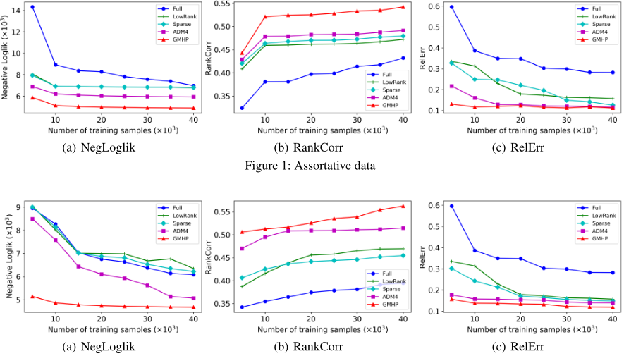
Figure 1 plots the results on assortative mixing data measured by NegLoglik, RankCorr, and RelErr with respect to the number of training data. It can be observed from the results that when the number of training samples increases, the RankCorr increases and both NegLoglik and RelErr decrease, indicating that all methods can improve accuracy of estimation with more training samples. Moreover, GMHP outperforms the baseline methods with all three metrics. We can see the prior graph structure knowledge can lead the learning of parameters and hence improve the estimation significantly. We can also see from the results that the improvements of GMHP are even larger when the sample sizes are small. This is because GMHP can leverage the prior graph structure knowledge, but the other methods may only integrate some assumptions about the influence patterns between events but no geographical or community information is considered. This feature of GMHP that can learn from fewer events makes GMHP effectively prevent over-fitting.
Similarly in Figure 2 GMHP outperforms other baseline methods on disassortative mixing data. These two experiments demonstrate that GMHP can effectively integrate the prior graph structure into learning.
Robustness
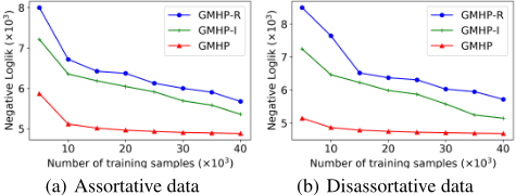
Figure 3(a) plots the results on assortative mixing data measured by NegLoglik with respect to the number of training data. It can be observed from the results that when the number of training samples increases, the NegLoglik decrease, indicating that all methods can improve accuracy of estimation with more training samples. At the same time, GMHP-R and GMHP-I still obtain stable performances even with random and incomplete connection matrices. Similarly in Figure 3(b) GMHP-R and GMHP-I obtain stable performances on disassortative mixing data. These two experiments demonstrate the robustness of GMHP.
4.5 Results on Real Data
We apply GMHP to model two real-world datasets, crime data and bike rental data, and compare it with Full, LowRank, Sparse, and ADM4.
Crime Data In this dataset, each police beat is considered as an event source, where each event indicates a crime record. To construct the connection matrix E for the crime data, we utilize the community information contained in the dataset. The beats are assigned to 77 communities, according to the activities of local residents. And we construct E by setting items between beats in the same community as 1, and 0 for others. We can say the beats in the same community are more related than the beats outside the community.
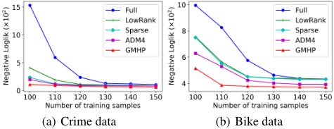
In total we have 196 months' data, and we learn the models from the first n months and test them on the data from the n + 1 month. Similar to the experiments on synthetic data, we obtain the NegLoglik with respect to different training periods which is shown in Figure 4(a). From the results we can see GMHP obtains better performance than other baseline methods.
Bike Data In this dataset, each bike station is considered as an event dimension/source, where each event indicates a renal transaction. To construct the connection matrix E for the bike data, we count start/end station pairs in bike rental transactions. We construct a network, with the bike stations as nodes, and the number of transactions as weights of edges between node pairs. Then a modularity-based community detection method is used to detect communities between stations. The stations in the same community are more related than the stations outside the community.
In total we have 180 days' data, and we we learn the models from the first n days and test them on the data from the n + 1 days. Similar to the experiments on synthetic data and criminal data, we obtain the NegLoglik with respect to different training periods which is shown in Figure 4(b). From the results we can see GMHP obtains better performance than other baseline methods.
In real applications, there may not have many events collected, for example, the crime events in a city happening everyday is limited. And that's also the reason why our proposed GMHP can be much useful in real applications with small number of events collected.
5 Conclusion
In this paper, we developed a framework for modeling spatiotemporal events with graph regularized multi-dimensional Hawkes process (GMHP). In the proposed GMHP framework, a graph regularization method was designed to integrate the prior spatial structure into MHP for learning influence matrix between different locations. Specifically, the prior spatial structure is first represented as a connection graph. Then, a multi-view method is utilized for the alignment of the prior connection graph and influence matrix while preserving the sparsity and low-rank properties of the kernel matrix. Moreover, we developed an optimization scheme using Alternating Direction Method of Multipliers (ADMM) to solve the resulting optimization problem. Finally, the experimental results have shown that our method can learn the interaction patterns between different geographical areas with prior connection graph introduced for regularization, and GMHP can effectively model spatio-temporal events.
@inproceedings{ijcai2018p343,
  title     = {Exploiting Graph Regularized Multi-dimensional Hawkes Processes for Modeling Events with Spatio-temporal Characteristics},
  author    = {Liu, Yanchi and Yan, Tan and Chen, Haifeng},
  booktitle = {Proceedings of the Twenty-Seventh International Joint Conference on
               Artificial Intelligence, {IJCAI-18}},
  publisher = {International Joint Conferences on Artificial Intelligence Organization},
  editor    = {Jérôme Lang},
  pages     = {2475--2482},
  year      = {2018},
  month     = {7},
  note      = {Main track},
  doi       = {10.24963/ijcai.2018/343},
  url       = {https://doi.org/10.24963/ijcai.2018/343},
}
TY - CPAPER TI - Exploiting Graph Regularized Multi-dimensional Hawkes Processes for Modeling Events with Spatio-temporal Characteristics AU - Liu, Yanchi AU - Yan, Tan AU - Chen, Haifeng T2 - Proceedings of the Twenty-Seventh International Joint Conference on Artificial Intelligence, IJCAI-18 PB - International Joint Conferences on Artificial Intelligence Organization PY - 2018 SP - 2475 EP - 2482 DO - 10.24963/ijcai.2018/343 UR - https://doi.org/10.24963/ijcai.2018/343 ER -Copied
Machine-readable versions of this paper, for tools and AI agents:





