Model-based Multi-agent Policy Optimization with Adaptive Opponent-wise Rollouts

1 Introduction

Multi-agent reinforcement learning (MARL) has been recently paid much attention and preliminarily applied to various control scenarios including robot system, autonomous driving, resource utilization etc. [Du and Ding, 2020]. One main technical challenge MARL brings over single-agent reinforcement learning (SARL) is that the agents need to interact with other agents, and their returns depend on the behavior of all the agents, which usually requires a considerable amount of samples, i.e., high sample complexity.

In a general MARL setting, one agent can access the actions taken by other agents in any state through some communication protocol, without any knowledge of their specific policies [Tian et al., 2020]. In such a situation, we claim that the sample complexity in MARL comes from two parts: dynamics sample complexity and opponent sample complexity. To achieve some policy performance, dynamics sample complexity represents the number of interactions made with the environment dynamics while collecting the samples. On the other hand, opponent sample complexity, which is unique in MARL, represents the times of communications to access one opponent's action. Thus one goal of MARL is to find an effective policy with the two sample complexities being low.

In SARL scenarios, it is well known that model-based reinforcement learning (MBRL) can achieve lower dynamics sample complexity than model-free reinforcement learning (MFRL) empirically [Wang et al., 2019] or achieve at least competitive complexity theoretically [Jin et al., 2018]. Specifically, by building a dynamics model, the agent can also be trained with the model simulation samples and the ones collected from the environment, which can reduce the need for the environment samples [Luo et al., 2019]. In multi-agent scenarios, however, to utilize the dynamics model for data simulation, we need to ask for the opponents' actions through a communication protocol, which will count as the opponent sample complexity. Via building opponent models [He et al., 2016], we can replace the real opponents in the data simulation stage to reduce the opponent sample complexity.

In this paper, we investigate model-based methods for MARL and propose a novel method called Adaptive Opponentwise Rollout Policy Optimization (AORPO). Specifically, from the perspective of each ego agent 1 , we build a multi-agent environment model, which consists of a dynamics model and opponent models for each opponent agent. The multi-agent environment model can then be used to perform simulation rollout for MARL training to reduce both sample complexities. To our knowledge, however, in literature, there is no theoretical guidance regarding how to perform the multi-agent simulated rollouts. We provide a theoretical analysis about the upper bound of the return discrepancy w.r.t. policy distribution shift and the generalization errors of the environment dynamics and each opponent model. The upper bound reveals that when the environment dynamics model performs rollout with multiple opponents models, different magnitudes of opponent model errors may lead to different contributions to the compounding error of the multi-step simulated rollouts. Based on the theoretic analysis, we design the adaptive opponent-wise rollout scheme for our policy optimization algorithm, called AORPO, and prove its convergence under reasonable assumptions.

Experiments show that AORPO outperforms several stateof-the-art MARL methods in terms of sample efficiency in both cooperative tasks and competitive tasks.

1 In this paper, each studied agent is called ego agent while the other agents are called opponent agents. See Figure 2 for illustrations.

2 RelatedWork

There are two important training paradigms in MARL, i.e., centralized training with decentralized execution (CTDE) and fully decentralized training. Typical algorithms using CTDE paradigm are value function decomposition algorithms [Whiteson, 2018], which deal with the non-stationarity and creditassignment challenges by a centralized value function. Fully decentralized MARL algorithms include consensus learning over networked agents and communicating agents [Zhang et al., 2018; Qu et al., 2019]. In decentralized scenarios, where the agents can communicate with each other, Iqbal and Sha [2019] proposed a method that integrates the received messages to learn a value function and a policy. In this paper, we propose a fully decentralized training method with a communication protocol.

Opponent modeling [He et al., 2016] is a feasible solution to the non-stationarity problem in MARL, which models others' policies with interaction experience. Behavior cloning is a straightforward method to learn opponents' policies [Lowe et al., 2017]. More advances include recursive reasoning with variational inference [Wen et al., 2019], maximum-entropy objective [Tian et al., 2019], and modeling the learning process of opponents [Foerster et al., 2018] etc.

There are generally two major problems for model-based RL methods, i.e., model learning and model usage. For model learning, the most common solution is supervised learning [Nagabandi et al., 2018], or non-parametric methods such as Gaussian processes [Kamthe and Deisenroth, 2018]. For model usage, a policy can be derived by exploiting the model with different algorithms such as Dyna [Sutton, 1990], shooting methods [Chua et al., 2018] and policy search with backpropagation through paths [Clavera et al., 2020]. We refer to Wang et al. [2019] for details of model-based RL. Theoretical analysis of model-based RL in single-agent scenarios has been investigated in recent literature. To name a few, Luo et al. [2019] provided a monotonic improvement guarantee by enforcing a distance constraint between the learning policy and the data-collecting policy. Janner et al. [2019] derived a return discrepancy bound with the branched rollout, which studies how the model generalization affects the model usage.

For model-based MARL, there are relatively limited works of literature, to our knowledge. Park et al. [2019] proposed to use a centralized auxiliary prediction network to model the environment dynamics to alleviate the non-stationary dynamics problem. Kamra et al. [2020] and Li et al. [2020] proposed interaction graph-based trajectory prediction methods, without considering policies. Krupnik et al. [2019] built a centralized multi-step generative model with a disentangled variational auto-encoder to predict the environment dynamics and the opponent actions and then performed trajectory planning. Unlike previous work, in our proposed AORPO each agent builds its environment model consisting of a dynamics model and opponent models, then learns its policy using the model rollouts. To our knowledge, AORPO is the first Dyna-style method in MARL. More importantly, AORPO is supported by the theoretical bound of return discrepancy and convergence guarantee, which provides a principle to design further Dyna-style model-based MARL methods.

3 ProblemDefinition and Sample Complexity 3.1 ProblemDefinition

We formulate the MARL problem as a stochastic game [Shapley, 1953]. An n-agent stochastic game can be defined as a tuple (S,A1 , . . . ,An ,R1 , . . . ,Rn , T , γ), where S is the state space of the stochastic game, Ai is the action space of agent i ∈ {1, . . . , n}, A = Πni=1Ai is the joint action space, Ri : S × A ↦→ R is the reward function of agent i, and γ is the discount factor. State transition proceeds according to the dynamics function T : S ×A ↦→ S. For agent i, denote its policy as πi : S → ∆(Ai ), which is a probability distribution over its action space, and πi (at|st) is the probability of taking action at at state st. By denoting other agents' actions as a-i = {aj }j̸=i, we can formulate the joint policy of other agents' as π-i (a-i t |st) = Πj∈{-i}πj (ajt |st). At each timestep, actions are taken simultaneously. Each agent i aims at finding its optimal policy to maximize the expected return (cumulative reward), defined as

We consider a general scenario that each ego agent i has no knowledge of other agents' policies, but can observe the histories of other agents, i.e., {s1:t-1, a-i 1:t-1 } at timestep t. This scenario is common in decentralized MARL, such as in Zhang et al. [2018] and Qu et al. [2019].

3.2 Two Parts of Sample Complexity

From the perspective of the ego agent i, the state transition in MARL involves sub-processes, i.e., the action sampling process π-i (a-i |s) of opponent agents given the current state s, and the transition process to the next state T (s′ |s, ai , a-i ) given the current state s and the joint action (ai , a-i ).

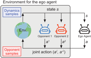
As such, for an ego agent to achieve some policy performance in a multi-agent environment, the sample complexity is specified in two parts: (i) dynamics sample complexity, i.e., the number of state transition interactions between the agent group and the dynamics environment, and (ii) opponent sample complexity, i.e., the total number of opponent action sampling given the conditioned state. Figure 1 illustrates such two parts of sample complexity.

We argue that it is necessary to study such two parts of sample complexity explicitly since the two sub-processes'

approximations meet different challenges. Environment dynamics modeling is usually computationally expensive as the state representation and the joint actions are usually of high dimensions. Opponent modeling usually aims at approximating the opponents' policies and eases MARL training in a decentralized manner [Tian et al., 2020].

Opponent Sample Complexity as Communication. If we leverage model-based techniques derived from SARL in multiagent cases with decentralized setting, we may need to call real opponents for the action given the current state, which can be formulated as a communication protocol. For example, the agents communicate via calling for the opponent actions [Tian et al., 2020]: the ego agent sends a state (no matter real or simulated) to an opponent agent and receives the action sampled from the opponent's policy. As such, we can regard the opponent sample complexity as communication load. To lower the opponent sample complexity, we replace the real opponents with learned opponent models in data simulation, which is analogous to selectively call some (or none) of opponents for useful information to reduce the communication load (or bandwidth) in multi-agent interactions [Ryu et al., 2020].

4 Return Discrepancy Bounds

In this section, we conduct theoretical analysis to better understand model-based MARL in the decentralized setting, where each ego agent learns a dynamics model and opponent models based on observed data. For a comprehensive analysis, we also discuss the bound in centralized model-based MARL in Appendix A 2 .

Usually, the dynamics model and opponent models have prediction errors, known as generalization errors. We investigate the influence of the learned models over the agent's performance. From the perspective of agent i, we aim to bound the discrepancy between the expected return ηi[πi , π-i ] of running the agent's policy πi in the real dynamics T with real opponents π-i and the expected return ˆ ηi[πi , ˆπ-i ] on a learned dynamics model ˆ T (s′ |s, ai , a-i ) with opponent models ˆπ-i . The return discrepancy upper bound C can be expressed as

Once the upper bound C is derived, it may indicate the key influence from the dynamics model and the opponent models, and thus helps design model-based algorithms accordingly.

In MARL with iterative policy optimization, we denote data-collecting policies in the previous iterations as (πiD , π-i D ). Then we measure the distribution shift between the current policies and the data-collecting policies with the total variation distance ϵiπ = maxs DTV (πi (·|s)‖πiD (·|s)), and similarly for the opponent agent j ∈ {-i}. Besides, interacting with (πiD , π-i D ), we denote the generalization error of the learned dynamics model ˆ T compared to the real environment dynamics T as ϵm = maxt E(st,ait ,a-i t )∼πiD ,π-i D [DTV (T (·|st, ait , a-i t )‖ ˆ T (·|st, ait , a-i t ))] and the error of the opponent model for agent j as ϵjˆπ = maxs DTV (πj (·|s)‖ ˆπj (·|s)). Now we are ready to provide an upper bound.

2 The full version of this paper with a detailed appendix can be found at https://arxiv.org/abs/2105.03363.

Theorem 1. Assume that the error of the learned dynamics model is bounded at each timestep by ϵm, and the distance of the policies are bounded by ϵiπ , ϵjπ , and the errors of the opponent models are bounded by ϵjˆπ , for j ∈ {-i}. The return discrepancy upper bound can be expressed as

Proof. The proof is provided in Appendix B.2.

□

This upper bound can be minimized by improving models' accuracy, which is the standard objective in previous literature. We investigate the model usage instead, and a more instructive and practical upper bound is needed.

Here we first investigate a k-step rollout scheme, which is a natural extension of MBPO [Janner et al., 2019] to multi-agent scenario. This rollout scheme begins from a state collected by the previous data-collecting policies, and then run the current policy for k steps under the learned dynamics model and the opponent models. Denoting the return of using multi-agent branched rollouts as ηbranch i , and the bound of the generalization error of the learned dynamics model with the current policies (πi , π-i ) as ϵ′m = maxt E(st,ait ,a-i t )∼πi ,π-i [DTV (T (·|st, ait , a-i t )‖ ˆ T (·|st, ait , a-i t ))] , we derive the following return discrepancy upper bound.

Theorem 2. Assume the generalization error is bounded by ϵ′m and the distance of the policies are bounded as ϵiπ , ϵjπ and ϵjˆπ for j ∈ {-i}. The bound of the discrepancy between the return in real environment ηi[πi , π-i ] and the return using the dynamics model and opponent models with branched rollouts ηbranch i [(π1D , ˆπ1 ), . . . , (πiD , πi ), . . . , (πnD , ˆπn )] is

where ϵ-i π = ∑j∈{-i} ϵjπ , ϵ-i ˆπ = ∑j∈{-i} ϵjˆπ and the pair (πjD , ˆπj ) means that the policy πjD and opponent model ˆπj are used before and after the branch point respectively for agent j.

The upper bound C(ϵ′m, ϵiπ , ϵ-i π , ϵ-i ˆπ , k) in Eq. (3) consists of the generalization errors of both dynamics model and opponent models as well as the policy distribution shift. Intuitively, choosing the optimal k∗ = argmink>0 C(ϵ′m, ϵiπ , ϵ-i π , ϵ-i ˆπ , k)

with sufficiently low ϵ′m and ∑j∈{-i} ϵjˆπ minimizes the discrepancy, which, however, cannot directly achieve a low discrepancy if any opponent model has relatively large error. So we need to reduce the upper bound such that the policy trained with the model rollouts will still perform well in real environment, leading to improved sample efficiency. To be more specific, we can optimize the target ηi through optimizing ηbranch i if the bound is tight. And improving ηbranch i by C(ϵ′m, ϵiπ , ϵ-i π , ϵ-i ˆπ , k) guarantees to improve the target ηi. It means that the policy improved under the environment model and the opponent models will get improved performance in the real environment.

Remark. As the policy is trained using mainly the samples from the model rollouts, which do not contribute to the sample complexity. A reduced return discrepancy upper bound indicates that the policy will get more improvement in the real environment given that the policy is improved to the same degree using the models. In other words, the policy will obtain the same performance improvement in the real environment with fewer samples with a reduced discrepancy upper bound.

Now the problem becomes how to reduce the bound in order to achieve low sample complexity. Considering that ϵjˆπ may be different across different opponent models, and sometimes the ego agent can call the real opponent agents for real actions, the rollout length k needs not to be the same across different opponents. Thus, in Section 5 we propose a method called Adaptive Opponent-wise Rollout Policy Optimization (AORPO) to reduce the upper bound.

5 The AORPOMethod

Based on the bound analysis in Theorem 2, now we present the detailed AORPO algorithm and prove its convergence.

5.1 AlgorithmDetails of AORPO

We propose a model-based MARL algorithm named MultiAgent Branched-Rollout Policy Optimization (AORPO). The overall algorithm of AORPO is shown in Algorithm 1. For simplicity, the detailed algorithm is described in the perspective of agent i. AORPO includes some key components, and the implementation of them is based on previous work, which serve as the preliminaries and are described in Appendix E.

In AORPO, the agent i learns a dynamics model and an opponent model for each of other agents and learns a policy based on the data collected from the model rollouts.

Agent Learning

For the dynamics model, in line 3 of Algorithm 1, a bootstrap ensemble of probabilistic dynamics models is trained to predict the environment dynamics as in Chua et al. [2018], and we select one of the models randomly from a uniform distribution when generating a prediction. For the opponent model, in line 6 of Algorithm 1, the policy of one opponent agent j can be modeled as a Gaussian distribution of the action. We further use the opponent models to encourage the coordination behaviors. Agent i makes a decision based on both the current state and the inferred opponent actions ˆa-i .

For the policy learning, AORPO is implemented based on the Multi-Agent Soft Actor-Critic (MASAC) algorithm,

Algorithm 1: AORPO Algorithm

• 1 Initialize policy πζ, Q value function Qω, predictive model ˆ Tθ, opponent models πφj for j ∈ {-i}, environment dataset Denv, model dataset Dmodel. 2 for N epochs do 3 Train model ˆ Tθ on Denv. 4 for E steps do 5 Take actions in environment via πζ with real opponents, add the transitions to Denv. 6 Train all opponent models πφj . 7 Compute the errors for each opponent model ϵjˆπ . 8 For each opponent, compute nj = ⌊k minj′ ϵj ′ ˆπ ϵjˆπ ⌋. 9 for M model rollouts do 10 Sample st uniformly fromDenv. 11 Perform k-step rollouts from st: 12 for p = 1, . . . , k do 13 ait+p-1 = πζ(st+p-1) 14 For each opponent j: 15 if p ≤ nj then 16 ajt+p-1 = πφj (st+p-1) 17 else 18 ajt+p-1 = Comm (st+p-1, j) 19 st+p = ˆ Tθ(st+p-1, ait+p-1 , a-i t+p-1 ) 20 Add the transitions to Dmodel. 21 Train the Q function and the policy using data fromDmodel with the loss in Eq. (5) and Eq. (4). 22 Function Comm (s, j) : 23 Send state s to agent j. 24 return the received aj

which is a multi-agent version of Soft Actor-Critic algorithm [Haarnoja et al., 2018]. In line 21 of Algorithm 1, agent i alternates between optimizing its policy and updating the value function. With the reparameterization function f and a Gaussian N, the policy optimization objective is

where D is the replay buffer, ϵt is the input noise and ˆa-i t ∼ ˆπ-i (·|st).

The loss function of the Q function is

where α is the temperature hyperparameter.

Adaptive Opponent-wise Rollout

In this work, a k-step model rollout begins from a real state collected in the real environment. We design the adaptive

Policy optimization

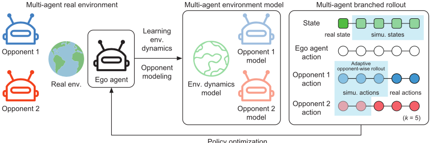
Figure 2: Illustration of the adaptive opponent-wise rollout policy optimization (AORPO) method from the perspective of the ego agent. The ego agent begins the rollouts from the states collected from the real environment interacting with real opponents, then runs k steps under the learned dynamics model. For each opponent agent, the ego agent interacts with it directly or with the opponent model for it in the k-step rollout, according to the prediction performance of its opponent model.

opponent-wise rollout scheme to reduce the bound. The opponent model generalization error term (k + 1) ∑j∈{-i} ϵjˆπ of the bound in Eq. (3) reveals that different magnitudes of opponent model errors may lead to different contributions to the compounding error of the multi-step simulated rollouts. Intuitively, if too short rollouts are performed, the relatively accurate opponent models are not fully utilized, leading to low sample efficiency. In contrast, if the rollout is too long, the relatively inaccurate opponent models may cause the rollouts to depart from the real trajectory distribution heavily, leading to degraded performance in the environment and thereby low sample efficiency. Thus our proposed adaptive opponent-wise rollout scheme lowers the rollout length of the relatively inaccurate opponent models but keeps long rollout length for relatively accurate opponent models, as shown in Figure 2.

We can achieve this since the agent i can play with either the learned opponent model ˆπj or the real policy πj of each opponent j. In detail, for the opponent j, ˆπj is used for the first nj = ⌊k minj′ ϵj ′ ˆπ ϵjˆπ ⌋ steps, then the agent i interacts with the real opponent πj in the rest k -nj steps. The compounding error contribution of each opponent model is thus bounded by kminj ′ ϵj ′ ˆπ . Note that the adaptive opponent-wise rollout scheme requires the ego agent i can obtain the actions ajt from the real policy in the last k - nj steps. In line 18 of Algorithm 1, the ego agent i sends the simulated states to the opponent j and requires the response, following the predefined communication protocol. One may argue that it will introduce extra opponent sample complexity since we need to communicate with the real opponent in the model rollouts. However, if we only use the opponent models, more errors are exploited, and it will lead to a poor policy and, finally, the sample complexity to achieve some good performance will be high. Our experiments in Section 6 will justify this claim.

With such nj 's, the generalization error caused by the opponent models becomes ∑j∈{-i} (nj + 1)ϵjˆπ ≃ (n - 1)kminj ′ ϵj ′ ˆπ , which is remarkably reduced and makes a good balance of the contribution to overall generalization error from different opponent models. According to the remark of Theorem 2, improving the surrogate return ηbranch i with a tighter discrepancy bound will improve the target return ηi more efficiently. Note that the comparison of different model usage schemes is provided in Appendix G.6, where the above scheme yields the highest asymptotic performance and sample efficiency.

5.2 Convergence Guarantee

According to Wei et al. [2018], the optimal policy learned by MASQL is π∗MASQL = exp ( 1α Q∗ (st, ·) -V ∗ (st)) = exp ( 1α Q∗ (st, ·))/ exp (V ∗ (st)), where Q∗ and V ∗ are the optimal Q function and state value function respectively. As Haarnoja et al. [2018] showed, the optimal policy learned by MASAC should be π∗MASAC = exp ( 1α Q∗ (st, ·))/Z(st). Since the partition function is Z(st) = exp (V ∗ (st)), with given the same optimal Q∗ and V ∗ , MASQL is equivalent to MASAC from the perspective of policy learning. With this fact, we prove that (1) using the learned dynamics model and the opponent models in AORPO still guarantees the convergence of MASQL; (2) MASQL still guarantees the convergence of Nash Q-learning [Hu and Wellman, 2003]. Thus we prove that AORPO achieves the convergence solution of Nash Qlearning. The theorems and proofs can be found in Appendix D, Theorem 6 and Theorem 7.

The theorems guarantee AORPO's convergence under several assumptions. However, we show that the assumptions are not necessary conditions for the learning algorithm to converges by the following experimental results in Figure 4, in which the convergence is still guaranteed when the assumptions are not strictly satisfied. More empirical findings can be found in Yang et al. [2018].

6 Experiments

We evaluate the performance of AORPO in both competitive and cooperative tasks. We demonstrate that AORPO can converge to the Nash equilibrium and that AORPO is more sample-efficient than a series of baselines in both competitive and cooperative tasks. See Appendix G for task details.

Compared Methods. We compare our method AORPO with the strong model-free MARL algorithms, MADDPG

[Lowe et al., 2017] and MASAC. To show that our multiagent models approach is generally helpful and to have fair comparisons, we also implement AORPO on top of MADDPG, named as AORDPG, for more comprehensive analysis.

Implementation. As for the practical implementation of AORPO, we first collect real experience data using model-free algorithms and use them to pre-train the dynamics model and the opponent models. Other implementation details, including network architectures and important hyperparameters, are provided in Appendix F.

6.1 Competitive Tasks

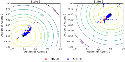
Climb is a modified Battle of Sex game. Agent 1 picks a number a ∈ [-1, 1], and agent 2 picks a number b ∈ [-1, 1]. Their actions form a position (a, b). There are 2 states and 2 corresponding landmarks located in the lower-left (-0.5,-0.5) and in the upper right (0.5, 0.5) respectively. The only Nash equilibrium is that the agents go to the lower-left landmark at state 1 and go to the upper right landmark at state 2.

The reward surfaces of converged MASAC and AORPO for the two agents in the two states are shown in Figure 4. The result verifies that AORPO will converge to the Nash equilibrium. In Appendix G.3 and G.4, we further provide more detailed results of comparing model-based and modelfree methods conducted in several competitive environments of the Multi-Agent Particle Environment [Lowe et al., 2017]

and the results of comparing AORPO with another modelbased MARL, i.e., MAMSGM [Krupnik et al., 2019].

6.2 Cooperative Tasks

Based on a multi-agent particle environment, we evaluate our method in two types of cooperative tasks: CESO tasks for complex environment dynamics and simple opponents, while SECO tasks for simple environment dynamics and complex opponents. CESO tasks include Cooperative communication with two agents and three landmarks and Cooperative navigation with three agents and three landmarks. The studied SECO task is Cooperative scheduling with three agents and three landmarks, as detailed in Appendix G.

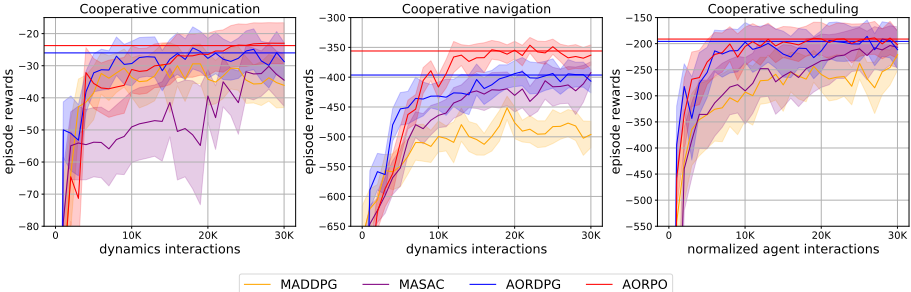
The laws of mechanics and the collisions' stochastic outcomes make difficulties for the dynamics model prediction, so we mainly consider the efficiency of interacting with the environment in the CESO tasks. In the left and middle subfigures of Figure 3, both AORPO and AORDPG can reach the asymptotic performance of the state-of-the-art model-free baselines with fewer interactions with the environment, i.e., achieving lower dynamics sample complexity.

The Cooperative scheduling task is configured as a SECO task, with two kinds of agents and two kinds of action spaces. We consider the efficiency of interacting with the other agents in the SECO tasks. As shown in the right subfigure of Figure 3, our methods AORPO and AORDPG reach the asymptotic performance with fewer agents' interactions, which means the opponent sample complexity is lower. One may think using opponent models will indeed introduce extra agent interactions when running rollouts, but interestingly, AORPO uses fewer agent interactions to achieve some performance since it helps policy learn faster. More detailed experiments are presented in Appendix G.

6.3 Analysis onModel Usage

We further discuss the effect of the opponent model usage. Although the generalization errors caused by the opponent models in the return discrepancy are hard to estimate, the opponent models affect the performance through the model compounding errors. We investigate the model compounding errors when using adaptive opponent-wise rollout or using the opponent models in a whole rollout. Specifically, for a real trajectory (s0, a0, . . . , sh), a branched rollout from the start state s0 under learned dynamics model and opponent models is denoted as (s0, ˆa0, . . . , ˆ sh). Following Nagabandi et al. [2018], the model compounding error is defined as ϵc = 1h ∑hi=1 ‖si - ˆ si‖22 .

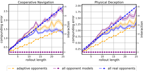
Using opponent models reduces interactions among agents but causes extra compounding errors compared with real opponents. We show the trade-off between model errors and interaction times in Figure 5, where the left and right y-axes are for the solid lines and the dotted lines, respectively. We observe the adaptive opponent-wise rollout achieves lower model compounding error than rollout with all opponent models while reducing the number of interactions compared to rollout with real opponents.

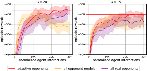
Moreover, we investigate how different rollout schemes affect the sample efficiency. In Figure 6, we compare three kinds of usages in a Cooperative navigation scenario using two settings of rollout length k. We notice that using the adaptive opponent-wise rollout achieves the same performance with fewer interactions among the agents than interacting with all real opponents, verifying that although we introduce some sample complexity while simulating data, the reduced discrepancy bound ensures the model-based methods to improve the sample efficiency. It can also avoid performance drop caused by compounding error compared with using all opponent models, which means that the adaptive opponent-wise rollout scheme mitigates some bad opponent models' negative effect by leveraging different rollout lengths of opponent models.

7 Conclusion

In this paper, we investigated model-based MARL problems with both theoretical and empirical analyses. We specified two parts of sample complexity in MARL and derived an upper bound of the return discrepancy in model-based MARL w.r.t. the policy distribution shift and the generalization errors of the learned dynamics model and opponent models. Inspired by the theoretical analysis, we designed the AORPO algorithm framework, in which the return discrepancy can be reduced by adaptive opponent-wise rollout controlling and the two parts of sample complexity are strategically reduced by the learned dynamics and opponent models. We then proved that AORPO can converge to Nash Q-values with reasonable assumptions. In experiments, AORPO has shown highly comparable asymptotic performance with the model-free MARL baselines while achieving higher sample efficiency. For future work, we plan to look deeper into various adaptive opponent-wise rollout schemes for different settings of model-based MARL. We will also investigate theoretical and empirical results of multi-agent dynamics model learning to further ease model-based MARL and improve its sample efficiency.

Acknowledgements

This work is supported by "New Generation of AI 2030" Major Project (2018AAA0100900) and National Natural Science Foundation of China (62076161, 61632017). Xihuai Wang is supported by Wu Wen Jun Honorary Doctoral Scholarship, AI Institute, Shanghai Jiao Tong University. We thank Yaodong Yang for helpful discussion.