
Blocking-based Neighbor Sampling for Large-scale Graph Neural Networks
Proceedings of the Thirtieth International Joint Conference on Artificial Intelligence. Main Track. Pages 3307-3313.
https://doi.org/10.24963/ijcai.2021/455
Keywords
- Machine Learning: Relational Learning
- Data Mining: Mining Graphs, Semi Structured Data, Complex Data
- Machine Learning Applications: Big data; Scalability
Abstract
The exponential increase in computation and memory complexity with the depth of network has become the main impediment to the successful application of graph neural networks (GNNs) on large-scale graphs like graphs with hundreds of millions of nodes. In this paper, we propose a novel neighbor sampling strategy, dubbed blocking-based neighbor sampling (BNS), for efficient training of GNNs on large-scale graphs. Specifically, BNS adopts a policy to stochastically block the ongoing expansion of neighboring nodes, which can reduce the rate of the exponential increase in computation and memory complexity of GNNs. Furthermore, a reweighted policy is applied to graph convolution, to adjust the contribution of blocked and non-blocked neighbors to central nodes. We theoretically prove that BNS provides an unbiased estimation for the original graph convolution operation. Extensive experiments on three benchmark datasets show that, on large-scale graphs, BNS is 2X~5X faster than state-of-the-art methods when achieving the same accuracy. Moreover, even on the small-scale graphs, BNS also demonstrates the advantage of low time cost.
- [Bruna et al., 2014] Joan Bruna, Wojciech Zaremba, Arthur Szlam, and Yann LeCun. Spectral networks and locally connected net- works on graphs. In International Conference on Learning Rep- resentations, 2014.
- [Chen et al., 2018a] Jianfei Chen, Jun Zhu, and Le Song. Stochas- tic training of graph convolutional networks with variance reduc- tion. In International Conference on Machine Learning, 2018.
- [Chen et al., 2018b] Jie Chen, Tengfei Ma, and Cao Xiao. FastGC- N: fast learning with graph convolutional networks via impor- tance sampling. In International Conference on Learning Repre- sentations, 2018.
- [Chen et al., 2020a] Lei Chen, Zhengdao Chen, and Joan Bruna. On graph neural networks versus graph-augmented MLPs. CoR- R, abs/2010.15116, 2020.
- [Chen et al., 2020b] Ming Chen, Zhewei Wei, Bolin Ding, Yaliang Li, Ye Yuan, Xiaoyong Du, and Ji-Rong Wen. Scalable graph neural networks via bidirectional propagation. In Advances in Neural Information Processing Systems, 2020.
- [Chen et al., 2020c] Ming Chen, Zhewei Wei, Zengfeng Huang, Bolin Ding, and Yaliang Li. Simple and deep graph convolution- al networks. In International Conference on Machine Learning, 2020.
- [Chiang et al., 2019] Wei-Lin Chiang, Xuanqing Liu, Si Si, Yang Li, Samy Bengio, and Cho-Jui Hsieh. Cluster-GCN: an efficient algorithm for training deep and large graph convolutional net- works. In ACM SIGKDD International Conference on Knowl- edge Discovery & Data Mining, 2019.
- [Cong et al., 2020] Weilin Cong, Rana Forsati, Mahmut T. Kan- demir, and Mehrdad Mahdavi. Minimal variance sampling with provable guarantees for fast training of graph neural networks. In ACM SIGKDD International Conference on Knowledge Discov- ery & Data Mining, 2020.
- [Fey and Lenssen, 2019] Matthias Fey and Jan E. Lenssen. Fast graph representation learning with PyTorch Geometric. In In- ternational Conference on Learning Representations Workshop on Representation Learning on Graphs and Manifolds, 2019.
- [Gori et al., 2005] M. Gori, G. Monfardini, and F. Scarselli. A new model for learning in graph domains. In IEEE International Joint Conference on Neural Networks, 2005.
- [Hamilton et al., 2017] William L. Hamilton, Zhitao Ying, and Jure Leskovec. Inductive representation learning on large graphs. In Adavances in Neural Information Processing Systems, 2017.
- [Hu et al., 2020] Weihua Hu, Matthias Fey, Marinka Zitnik, Yux- iao Dong, Hongyu Ren, Bowen Liu, Michele Catasta, and Jure Leskovec. Open graph benchmark: datasets for machine learn- ing on graphs. In Advances in Neural Information Processing Systems, 2020.
- [Huang et al., 2018] Wen-bing Huang, Tong Zhang, Yu Rong, and Junzhou Huang. Adaptive sampling towards fast graph represen- tation learning. In Adavances in Neural Information Processing Systems, 2018.
- [Kingma and Ba, 2015] Diederik P. Kingma and Jimmy Ba. Adam: a method for stochastic optimization. In International Confer- ence on Learning Representations, 2015.
- [Kipf and Welling, 2017] Thomas N. Kipf and Max Welling. Semi- supervised classification with graph convolutional networks. In International Conference on Learning Representations, 2017.
- [Klicpera et al., 2019] Johannes Klicpera, Stefan Weißenberger, and Stephan Günnemann. Diffusion improves graph learning. In Adavances in Neural Information Processing Systems, 2019.
- [Li et al., 2018] Qimai Li, Zhichao Han, and Xiao-Ming Wu. Deep- er insights into graph convolutional networks for semi-supervised learning. In AAAI Conference on Artificial Intelligence, 2018.
- [Li et al., 2019] Guohao Li, Matthias Müller, Ali K. Thabet, and Bernard Ghanem. DeepGCNs: can GCNs go as deep as C- NNs? In IEEE/CVF International Conference on Computer Vi- sion, 2019.
- [Oono and Suzuki, 2020] Kenta Oono and Taiji Suzuki. Graph neu- ral networks exponentially lose expressive power for node clas- sification. In International Conference on Learning Representa- tions, 2020.
- [Paszke et al., 2019] Adam Paszke, Sam Gross, Francisco Massa, Adam Lerer, James Bradbury, Gregory Chanan, Trevor Killeen, Zeming Lin, Natalia Gimelshein, Luca Antiga, Alban Desmai- son, Andreas Köpf, Edward Yang, Zachary DeVito, Martin Raison, Alykhan Tejani, Sasank Chilamkurthy, Benoit Steiner, Lu Fang, Junjie Bai, and Soumith Chintala. Pytorch: an impera- tive style, high-performance deep learning library. In Adavances in Neural Information Processing Systems, 2019.
- [Velickovic et al., 2018] Petar Velickovic, Guillem Cucurull, Aran- txa Casanova, Adriana Romero, Pietro Liò, and Yoshua Bengio. Graph attention networks. In International Conference on Learn- ing Representations, 2018.
- [Verma and Zhang, 2020] Saurabh Verma and Zhi-Li Zhang. To- wards deeper graph neural networks. In ACM SIGKDD Inter- national Conference on Knowledge Discovery & Data Mining, 2020.
- [Wu et al., 2019] Felix Wu, Amauri H. Souza Jr., Tianyi Zhang, Christopher Fifty, Tao Yu, and Kilian Q. Weinberger. Simpli- fying graph convolutional networks. In International Conference on Machine Learning, 2019.
- [Xu et al., 2018] Keyulu Xu, Chengtao Li, Yonglong Tian, Tomohi- ro Sonobe, Ken-ichi Kawarabayashi, and Stefanie Jegelka. Rep- resentation learning on graphs with jumping knowledge network- s. In International Conference on Machine Learning, 2018.
- [Zeng et al., 2020] Hanqing Zeng, Hongkuan Zhou, Ajitesh Srivas- tava, Rajgopal Kannan, and Viktor K. Prasanna. GraphSAINT: graph sampling based inductive learning method. In Internation- al Conference on Learning Representations, 2020.
- [Zou et al., 2019] Difan Zou, Ziniu Hu, Yewen Wang, Song Jiang, Yizhou Sun, and Quanquan Gu. Layer-dependent importance sampling for training deep and large graph convolutional net- works. In Adavances in Neural Information Processing Systems, 2019.
References were extracted automatically from the PDF and may contain errors.
Full text extracted automatically from the PDF; figures, tables and equations may differ. The PDF is the version of record.
1 Introduction
Graph has been widely used for describing unstructured data in real applications such as social networks, brain networks, molecular graphs, and knowledge graphs. Edges in graphs depict the complex relationships between samples, and rich relational information between samples is contained in graphs. Making good use of the rich relational information between samples in graphs has great potential in boosting the performance of traditional machine learning methods which are mainly designed for modeling independent and identically distributed (i.i.d.) data. In addition, graph data is now widely available in many applications. Therefore, developing advanced graph learning algorithms is a topic of great inter- Among various algorithms of representation learning for graphs, graph neural networks (GNNs) [Gori et al., 2005; Bruna et al., 2014] have recently become the most successful and popular ones, due to their powerful ability in modeling complex relationships between samples. Although many advanced GNN models [Kipf and Welling, 2017; Hamilton et al., 2017; Velickovic et al., 2018] have been proposed, most of them are limited to the successful application on smallscale graphs (e.g., graphs with hundreds of thousands of nodes). There are significant challenges in applying existing GNN methods to applications with large-scale graphs (e.g., graphs with hundreds of millions of nodes) because of the expensive computation and memory cost during the training process. Due to the iteratively dependent nature of nodes in GNNs, the number of nodes supporting the computation of output layer exponentially increases with the depth of network. Hence, the computation and memory complexity grow exponentially. Moreover, recent works [Li et al., 2019; Verma and Zhang, 2020; Chen et al., 2020c] show the potential to improve the performance of GNN models as the network becomes deeper, which will undoubtedly exacerbate the problem of expensive cost on large-scale graphs. Nowadays, in order to speed up the training process, it is a dominant trend to perform training on GPUs. However, many GPUs have limited graphics memory, which hinders GNN models from training with large batch size and as a result leads to a sharp increase in time cost for training.
est.∗Corresponding author
Solutions for the above problem mainly include model simplification methods and sampling-based methods. For model simplification methods [Wu et al., 2019; Klicpera et al., 2019; Chen et al., 2020b], the main idea is to remove the nonlinear transformation between graph convolution layers such that the graph convolution on node features can be preprocessed before training. Although model simplification methods are efficient in training, as stated in [Chen et al., 2020a], it is still an open question whether simplified GNNs' expressive power can match that of the original GNNs. For sampling-based methods, existing works can be broadly categorized into node-wise sampling [Hamilton et al., 2017; Chen et al., 2018a; Cong et al., 2020], layer-wise sampling [Chen et al., 2018b; Huang et al., 2018; Zou et al., 2019], and subgraph sampling [Chiang et al., 2019; Zeng et al., 2020]. For node-wise sampling, the main idea is to sample a number of neighbors for each node of each layer in a top-down manner. For layer-wise sampling, the main idea is to independently sample a number of nodes from a candidate set for each layer based on the importance probabilities of nodes. All connections between the nodes of two adjacent layers are used to perform approximate graph convolution. For subgraph sampling, the main idea is to sample a subgraph and feed it to GNN models before each round of mini-batch training. Although the above sampling strategies are applicable to large-scale GNNs, they have some deficiencies or limitations in terms of accuracy, total time cost, or memory cost. For example, existing node-wise sampling strategies need to sample a large number of neighbors for high accuracy, which will lead to a sharp increase in time cost. Layer-wise sampling strategies have a high time cost of preparing data (including sampling) and may suffer from sparse connection between two adjacent layers. Subgraph sampling strategies may also suffer from sparse connection in subgraphs.
In this paper, we propose a novel node-wise sampling strategy, called blocking-based neighbor sampling (BNS), for large-scale training of GNNs. The contributions of this paper are listed as follows:
- We propose a novel blocking mechanism in BNS to stochastically block the ongoing expansion of neighboring nodes, dramatically reducing the computation and memory complexity.
- We further propose a reweighted policy to adjust the contribution of blocked and non-blocked neighboring nodes to central nodes.
- We theoretically prove that BNS provides an unbiased estimation for the original graph convolution operation.
- Extensive experiments on large-scale graphs show that BNS is 2× ∼ 5× faster than existing state-of-the-art methods when achieving the same accuracy. Even on the small-scale graph, BNS also demonstrates the advantage of low time cost.
2 Notations and ProblemDefinition
2.1 Notations
We use boldface uppercase letters, such as B, to denote matrices. The ith row and the jth column of a matrix B are denoted as Bi∗ and B∗j, respectively. Bij denotes the element at the ith row and jth column in B. ‖B‖0 denotes the number of non-zero entries in B. ‖B‖F denotes the Frobenius norm of B.
2.2 ProblemDefinition
Suppose we have a graph with N nodes. Let A ∈ {0, 1}N×N denote the adjacency matrix of the graph. Aij = 1 denotes there exists an edge between node i and node j, and Aij = 0 denotes there is no edge between them. Let X ∈ RN×u denote the node feature matrix, where u denotes the dimension of node feature. Suppose the average number of neighbors per node in the graph is s. Suppose the mini-batch size of nodes at output layer is B. We use L to denote the layer number of GNNs.
We take GCN [Kipf and Welling, 2017] as an example to describe the problem of the exponential increase in computation and memory complexity. Let A′ = A + I and ˆA = D- 1 2 A′D- 1 2 , where D denotes the diagonal degree matrix of A′ and Dii = ∑nj=1 A′ij . Then GCN can be formulated as follows:
where H(0) = X, f(·) is the activation function, N(i) denotes the set of neighbors of node i. W(ℓ) ∈ Rr×r is a learnable parameter.
From (1), we can see that the output of a node at the Lth layer iteratively depends on the information of its 1, · · · , Lhop neighbors. Such an iteratively dependent nature of nodes leads to the exponential increase in computation and memory complexity with the depth of network. Let r denote the feature dimension of hidden layer. Then, the computation and memory complexity during a mini-batch training are O(sL-1 · (sBr +Br2 )) and O(Lr2 + sL · Br), respectively.
3 Blocking-based Neighbor Sampling
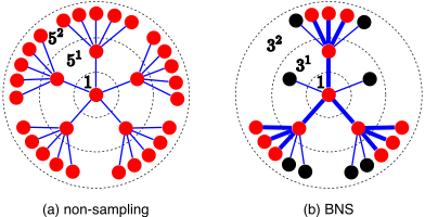
In this section, we present the details of BNS. Firstly, we sample a fixed number of neighbors for each node at the current layer ℓ. Secondly, we adopt a policy to stochastically block the ongoing expansion of neighboring nodes at the preceding layers {1, · · · , ℓ-1}. Note that once a node is blocked, all its ways out to all other nodes are blocked, and it is trapped at its current position. Thirdly, after sampling finishes, reweighted graph convolution is performed to obtain the outputs, in which a reweighted policy is adopted to adjust the contribution of blocked and non-blocked neighbors to central nodes. A visual illustration of BNS is presented in Figure 1.
3.1 Sampling Algorithm
The entire sampling process is performed in a top-down manner, and it is summarized in Algorithm 1. Suppose Vin denote a mini-batch of nodes in the output layer. Firstly, we sample sn neighbors for each node i at layer ℓ in line 5. Sample(N(i), sn) in line 5 is an operation that uniformly samples sn elements from N(i). Then, we randomly select sn × δ (0 ≤ δ ≤ 1) nodes from N ℓ (i) in line 6, and stop sampling neighbors for them at the preceding layers {1, · · · , ℓ - 1} via the operations in line 7 and line 13. Block(N ℓ (i), δ) in line 6 is an operation that uniformly samples |N ℓ (i)| × δ elements from N ℓ (i) as blocked neighbors. V ℓ b records the blocked nodes at the ℓth layer, which are used in subsequent processing steps. The operations in line 10 and line 11 ensure that the blocked nodes are mapped to the same feature space as non-blocked nodes.
3.2 Reweighted Graph Convolution
We first reformulate Z(ℓ) i∗ in Equation (1) to an expectation form:
where p(j ∈ N(i)|i) is a uniform distribution over the neighbors of node i. |N(i)| denotes the number of elements in N (i).
For blocked nodes, since their neighbor expansions are blocked, their estimation for Equation (2) is less precise (having large variance) than non-blocked nodes. We can see that representations of blocked nodes carry little information about the input graph. Therefore, it is reasonable to increase the contribution of non-blocked nodes to the central nodes. We perform reweighted graph convolution to achieve this goal.
After Algorithm 1 is performed, reweighted graph convolution is formulated as follows. For readability, we denote nℓi,1 = |N ℓ b (i)|, nℓi,2 = |N ℓnb (i)| and ni = |N(i)|.
where ρ ∈ [0, 1]. Compared with (|N(i)|/|N ℓ (i)|) · ˆ Aij in Equation (2), ˜ Aij adopts a different weights, ρℓi,1 and ρℓi,2 , to adjust the contribution of non-blocked and blocked nodes to node i. In the following proposition, we prove that ˜Z(ℓ) is an unbiased estimation of Z(ℓ) i∗ , which makes our proposed reweighted graph convolution theoretically sound. In experiments, ρ is set to 0.5 for convenience.
Proposition 1. Suppose H(ℓ-1) is given. If N ℓ (i) is uniformly sampled from N(i), N ℓ b (i) is uniformly sampled from N ℓ (i) and ρ ∈ [0, 1], then ˜Z(ℓ) i∗ defined in Equation (4) is an unbiased estimation of Z(ℓ) i∗ .
Proof. The proof can be found in the Appendix 1 .
1 The Appendix can be found in https://cs.nju.edu.cn/lwj/.
Algorithm 1 Sampling Algorithm
Require: Mini-batch of nodes Vin, the number of neighbors sampled for each node sn, ratio of blocked neighbors per node δ.
Ensure: {(V ℓnb , V ℓ b , {(N ℓnb (i), N ℓ b (i))}Ni=1 )}Lℓ=1
- 1: V L nb = Vin, Vb = ∅
- 2: Sample in a top-down manner:
- 3: for ℓ = L : 1 do
- 4: for i ∈ V ℓnb do
- 5: N ℓ (i) = Sample(N(i), sn)
- 6: N ℓ b (i) = Block(N ℓ (i), δ)
- 7: N ℓnb (i) = N ℓ (i)\N ℓ b (i)
- 8: end for
9:
- 10: N ℓ (i) =N ℓ (i) ∪ {i}
for i ∈ Vb do
- 11: N ℓ b (i) = N ℓ b (i) ∪ {i}
- 12: end for
- 13: V ℓ-1 nb = ⋃i∈V ℓnb N ℓnb (i)
- 14: V ℓ-1 b = ⋃i∈V ℓnb N ℓ b (i)
- 15: Vb = Vb ∪V ℓ-1 b
- 16: end for
3.3 Objective Function
Let W = {W(1) , · · · ,W(L) } denote the learnable parameters defined in Equation (5). ˆY = H(L) denotes the output of GNN models. For multi-class classification, f(·) in the last layer denotes the softmax function, while it denotes the sigmoid function for multi-label classification. The objective function for BNS is formulated as follows:
where λ is a hyper-parameter for the regularization term of parameters W, V ′ denotes the set of nodes in training set.
3.4 Complexity Analysis
In this subsection, we compare the computation and memory complexity of different methods with those of BNS in a mini-batch training step, which is summarized in Table 1. For existing node-wise sampling methods NS [Hamilton et al., 2017], VRGCN [Chen et al., 2018a] and MVS-GNN [Cong et al., 2020], they reduce the growth rate from s to sn, where sn is much smaller than s. In particular, VRGCN and MVS-GNN show that they can achieve comparable accuracy to NS with smaller sn. For layer-wise sampling method LADIES [Zou et al., 2019] and subgraph sampling method GraphSAINT [Zeng et al., 2020], they reduce the computation and memory complexity to the level that is linear with the depth of network.
Although the above methods can achieve good performance in terms of accuracy, time cost, and memory cost on small-scale graphs (e.g., graphs with hundreds of thousands of nodes), they are not efficient or even not applicable for large-scale graphs (e.g., graphs with millions of nodes and hundreds of millions of nodes). Some problems and drawbacks existing in these methods are overlooked due to the lack of systematically experimental analysis on large-scale graphs. For example, even with low computation complexity, VRGCN, MVS-GNN and LADIES have a high time cost of preparing data (including sampling) before each round of mini-batch training. In addition, VRGCN brings a huge burden to the memory for storing all nodes' historical representations at each layer. MVS-GNN has the same complexity as the non-sampling method at the outer iteration, which might make the training infeasible on large-scale graphs because of running out of graphics memory. GraphSAINT faces the problem of sparse connection in subgraphs. Moreover, GraphSAINT adopts the non-sampling strategy at the evaluation and testing stage, which is also inefficient on large-scale graphs.
| Method | Computation complexity | Memory complexity |
|---|---|---|
| Non-sampling [Kipf and Welling, 2017] NS [Hamilton et al., 2017] VRGCN [Chen et al., 2018a] MVS-GNN [Cong et al., 2020] LADIES [Zou et al., 2019] GraphSAINT [Zeng et al., 2020] | O(sL-1 (sBr + Br2 )) O(sL-1 n · (snBr +Br2 )) O(sL-1 n · ((sn + s) · Br +Br2 )) O(sL-1 n · ((sn + s) · Br +Br2 )) O(L · (sl/N)2 · ‖A‖0 +Lsl · r2 ) O(L · (sg/N)2 · ‖A‖0 +Lsg · r2 ) | O(Lr2 + sL · Br) O(Lr2 + sLn · Br) O(Lr2 + sL-1 n · (s + sn)Br) O(Lr2 + sL-1 n · (s + sn)Br) O(Lr2 +Lsl · r) O(Lr2 +Lsg · r) |
| BNS (ours) | n · (snBr + (δ/(1 - δ) +1) · | + ˜ n · |
| O(˜ sL-1 Br2 )) | O(Lr2 sL-1 snBr) |
Similar to existing node-wise sampling methods, BNS reduces the growth rate from s to a small ˜ sn, where ˜ sn denotes the number of non-blocked neighbors per node. We will show that with a small ˜ sn, BNS can achieve comparable accuracy to NS with a large sn, while BNS has lower computation and memory complexity. Moreover, BNS has a low time cost of preparing data before each round of mini-batch training.
4 Experiments
In this section, we compare BNS with other baselines on five node-classification datasets. BNS is implemented on the Pytorch platform [Paszke et al., 2019] with Pytorch-Geometric Library [Fey and Lenssen, 2019]. All experiments are run on a NVIDIA TitanXP GPU server with 12 GB graphics memory.
4.1 Datasets
Ogbn-products, ogbn-papers100M and ogbn-proteins 2 are publicly available [Hu et al., 2020]. Ogbn-products is a largescale dataset with millions of nodes. Ogbn-papers100M is a large-scale dataset with hundreds of millions of nodes. Ogbnproteins is a small-scale dataset with hundreds of thousands of nodes. Amazon and Yelp in GraphSAINT, are also used for evaluation. Due to space limitation, the information and results on Amazon and Yelp are moved to the Appendix. The statistics of datasets can be found in the Appendix.
2 https://ogb.stanford.edu/docs/nodeprop/
4.2 Baselines and Settings
We compare BNS with VRGCN [Chen et al., 2018a], LADIES [Zou et al., 2019] and GraphSAINT [Zeng et al., 2020], which are the state-of-the-art methods with node-wise sampling, layer-wise sampling and subgraph sampling, respectively. Additionally, we compare BNS with the classical node-wise sampling method NS [Hamilton et al., 2017]. We do not compare BNS with MVS-GNN since MVS-GNN adopts the non-sampling strategy for training at the outer iteration, which leads to the problem of running out of graphics memory. Besides, comparisons with model simplification methods are moved to the Appendix due to space limitation. Since the original implementations of the above baselines cannot directly scale to the benchmark datasets in this paper, we re-implement them according to the corresponding authors' codes. For a fair comparison, implementations of all methods, including BNS, only differ in the sampling process. For all methods, GNN model is instantiated with GraphSAGE [Hamilton et al., 2017], since it can achieve good performance on the benchmark datasets. Note that sampling strategies and settings during inference are the same as those in the training stage for all methods except for GraphSAINT.
The hyper-parameters r, L, T (maximum epoch), λ and p (probability of dropout) are independent of sampling strategies, and hence they are set to be the same for different sampling strategies on one specific dataset. Empirically, r is set to 128 on all datasets, L is set to 5 on both ogbn-proteins and ogbn-products, and L is set to 3 on ogbn-papers100M. For T , it is set to 100 on both ogbn-products and ogbn-papers100M, and set to 1,000 on ogbn-proteins. For λ and p, the values of them are obtained by tuning with NS on the benchmark datasets. On ogbn-product, λ = 5 × 10⁻⁶ and p = 0.1. On ogbn-papers100M, λ = 5 × 10⁻⁷ and p = 0.1. On ogbnproteins, λ = 0 and p = 0. In BNS, we set ρ to 0.5 for convenience and do not tune it. Adam [Kingma and Ba, 2015] is used to optimize the model and the learning rate η is set to 0.01. For all settings, experiments are run for 10 times with different initialization each time, and the mean results of 10 runs are reported.
4.3 Evaluation Criteria
The ultimate goal of sampling strategies for GNNs is to obtain high accuracy with a low time cost, not just to reduce time and memory cost to extreme cases at the expense of sac-
(b) ogbn-papers100M.
| Methods | ogbn-products | ogbn-papers100M | ||||
|---|---|---|---|---|---|---|
| Accuracy (%) ↑ | Time (s) ↓ | T1+T2 (s) | Accuracy (%) ↑ | Time (s) ↓ | T1+T2 (s) | |
| NS | 78.64 ± 0.17 | 5.5×10³ | 4.5 ×10³ +9.6×10² | 63.61 ± 0.13 | 2.5×10⁴ | 8.0×10³ +1.7×10⁴ |
| VRGCN | 77.07 ± 0.49 | 1.2×10⁴ | 1.1 ×10⁴ +1.5×10³ | 63.34 ± 0.12 | 2.2×10⁴ | 7.0×10³ +1.5×10⁴ |
| LADIES | 78.96 ± 0.50 | 4.7×10³ | 4.5 ×10³ +2.5×10² | 63.25 ± 0.21 | 2.5×10⁴ | 1.2×10⁴ +1.3×10⁴ |
| GraphSAINT | 78.95 ± 0.41 | 7.1 ×10³ | 4.5×10³ +2.6×10³ | 61.60 ± 0.12 | 2.1×10⁴ | 8.0×10³ +1.3×10⁴ |
| BNS (ours) | 80.14 ± 0.27 | 9.1×10² | 7.3 ×10² +1.8×10² | 63.88 ± 0.12 | 1.2×10⁴ | 4.3×10³ +7.7×10³ |
Table 2: Results on ogbn-products and ogbn-papers100M. Boldface letters denote the best results. Time presented in tables denotes the total training time of one run. "T1" refers to the time cost of preparing data. "T2" refers to the time cost of performing forward and backward propagation. The results in tables are obtained under the second experimental setting in the Section 4.3.
rificing accuracy. In most cases, reducing memory can also reduce the time cost since GNN model can perform training with a larger batch size when the graphics memory cost is lower. Hence, we omit the comparison of memory cost in experiments. In a nutshell, the accuracy of GNN model and time cost during training are presented to evaluate the performance of different methods.
One reasonable way to evaluate the performance of different methods is to compare time cost when achieving the same accuracy. Since batch size has an important impact on time cost and accuracy, we design two kinds of experiments for fair comparison:
- The first experimental setting: On each dataset, for different methods, we train GNN model with the same batch size. All methods are run with the best setting that can achieve the best accuracy in this case.
- The second experimental setting: On each dataset, for different methods, we train GNN model with the maximum batch size that can achieve the best accuracy. All methods are run with the best setting that can achieve the best accuracy.
Detailed settings of each method can be found in the Appendix.
4.4 Results
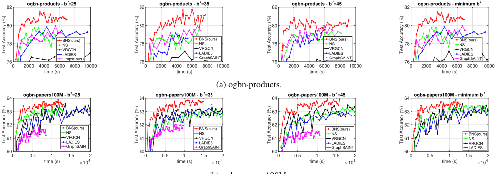
Results on ogbn-products and ogbn-papers100M are summarized in Figure 2 and Table 2, from which we can draw the following conclusions. Firstly, when achieving the same accuracy under different settings, BNS is faster than all other methods. For example, from Figure 2(a), we can see that BNS is approximately 4× ∼ 5× faster than GraphSAINT (secondbest) when achieving the accuracy of 80% on ogbn-products. From Figure 2(b), we can see that BNS is approximately 2× faster than NS (second-best) when achieving the accuracy of 63.5% on ogbn-papers100M. Secondly, compared with other methods, BNS can achieve the best performance in accuracy with the minimum time cost. This point can be drawn from Table 2, which is consistent with the results in Figure 2. Thirdly, VRGCN and LADIES have a high time cost in preparing data, which is even higher than the time cost in performing forward and backward propagation. Finally, from Table 2, we observe an interesting phenomenon, i.e., the accuracy of BNS does not decrease compared to that of NS, and is even higher than that of NS. This phenomenon can be explained by the observations in JK-Net [Xu et al., 2018], i.e., it is important to enhance the influence of local neighborhoods on the central nodes; otherwise the local information of the central nodes in the input graphs will be washed out in a few
80
Test ROC-AUC (%)
78
76
74
ogbn-proteins - b =35
BNS(ours)
NS
VRGCN
LADIES
GraphSAINT
0
0.5
1
1.5
2
time (s)
10 4
| Method | Accuracy (%) ↑ | Time (s) ↓ | T1+T2 (s) |
|---|---|---|---|
| NS | 78.84 ± 0.32 | 1.1 ×10⁴ | 3.6×10³ +7.4×10³ |
| VRGCN | 78.26 ± 0.64 | 1.9 ×10⁴ | 8.0×10³ +1.1×10⁴ |
| LADIES | 79.49 ± 0.37 | 1.9×10⁴ | 1.9×10⁴ +3.0×10² |
| GraphSAINT | 78.73 ± 0.45 | 3.3×10⁴ | 1.1×10⁴ +2.2×10⁴ |
| BNS (ours) | 79.60± 0.29 | 9.3×10³ | 8.6×10³ +7.4×10² |
steps. We can see that the stochastically blocking policy is helpful for BNS to preserve local information around central nodes.
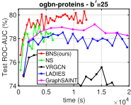
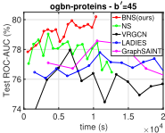
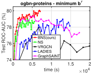
Results on ogbn-proteins, a relative small graph, are summarized in Figure 3 and Table 3, from which we can draw the following conclusions. Firstly, BNS is faster than all other methods when achieving the same accuracy under different settings. However, the gap of the time cost for achieving the same accuracy between BNS and other methods is small. The main reason is that neighboring expansions can easily cover the entire graph within a few layers or steps on small-scale graphs. Therefore, these methods have the same order of computation and memory complexity O(Nsr +Nr2 ). Secondly, BNS can achieve the best performance in terms of accuracy with the fastest speed. This point can be drawn from Table 3, which is consistent with results in Figure 3. Thirdly, once again, we observe that LADIES has a high time cost in preparing data. Finally, we observe that GraphSAINT (non-sampling strategy) achieves lower accuracy than NS, LADIES and BNS. This may be caused by the over-smoothing problem of GNNs [Li et al., 2018; Xu et al., 2018; Oono and Suzuki, 2020]. This observation, in turn, shows that the stochasticity introduced by sampling can alleviate the over-smoothing problem of GNNs.
Summary. First, on large-scale graphs, BNS is 2× ∼ 5× faster than existing state-of-the-art methods when achieving the same accuracy. Compared with BNS, other methods have some deficiencies or limitations. For example, NS needs a large number of sn to achieve high accuracy. VRGCN and LADIES have a high time cost of preparing data, which are more expensive than performing forward and backward propagation. Second, even on the small-scale graph, BNS demonstrates the advantage of low time cost. Third, compared with other methods, BNS can achieve the best performance in accuracy with the minimum time cost.
4.5 Ablation Study
We study the effectiveness of reweighted policy by setting ρℓi,1 = 1 and ρℓi,2 = 1 in Equation (3). With ρℓi,1 = 1 and
ρℓi,2 = 1 in Equation (3), Equation (5) is a plain Monte-Carlo approximation of Equation (2). The results are presented in Table 4. From Table 4, we can conclude that reweighted policy enhances the ability of BNS in utilizing the information of blocked neighbors.
| Accuracy (%) or ROC-AUC (%) | |||
|---|---|---|---|
| Methods | ogbn- products | ogbn- papers100M | ogbn- proteins |
| BNS w/o rew | 79.12 ± 0.19 | 62.54 ± 0.14 | 79.40 ± 0.21 |
| BNS | 80.14 ± 0.27 | 63.88 ± 0.12 | 79.60 ± 0.29 |
5 Conclusions
On large-scale graphs (e.g., graphs with hundreds of millions of nodes), existing sampling strategies have deficiencies or limitations in accuracy, time cost, or memory cost. Hence, designing an effective sampling strategy for efficient training of GNNs on large-scale graphs is still challenging. In this paper, we propose a novel neighbor sampling strategy, dubbed blocking-based neighbor sampling (BNS), for training GNNs on large-scale graphs. The main idea is to adopt a policy to stochastically block the ongoing expansion of neighbors, by which computation and memory complexity can be significantly reduced. Furthermore, reweighted graph convolution is proposed to adjust the contribution of blocked and nonblocked neighbors to central nodes. Extensive experiments on large-scale graphs show that, when achieving the same accuracy, BNS is 2× ∼ 5× faster than state-of-the-art methods. Experiments on the small-scale graph also demonstrate the advantage of BNS in terms of time cost.
Acknowledgments
This work is supported by the NSFC-NRF Joint Research Project (No. 61861146001) and NSFC Project (No. 61921006).
@inproceedings{ijcai2021p455,
  title     = {Blocking-based Neighbor Sampling for Large-scale Graph Neural Networks},
  author    = {Yao, Kai-Lang and Li, Wu-Jun},
  booktitle = {Proceedings of the Thirtieth International Joint Conference on
               Artificial Intelligence, {IJCAI-21}},
  publisher = {International Joint Conferences on Artificial Intelligence Organization},
  editor    = {Zhi-Hua Zhou},
  pages     = {3307--3313},
  year      = {2021},
  month     = {8},
  note      = {Main Track},
  doi       = {10.24963/ijcai.2021/455},
  url       = {https://doi.org/10.24963/ijcai.2021/455},
}
TY - CPAPER TI - Blocking-based Neighbor Sampling for Large-scale Graph Neural Networks AU - Yao, Kai-Lang AU - Li, Wu-Jun T2 - Proceedings of the Thirtieth International Joint Conference on Artificial Intelligence, IJCAI-21 PB - International Joint Conferences on Artificial Intelligence Organization PY - 2021 SP - 3307 EP - 3313 DO - 10.24963/ijcai.2021/455 UR - https://doi.org/10.24963/ijcai.2021/455 ER -Copied
Machine-readable versions of this paper, for tools and AI agents:





