
Sensitivity Direction Learning with Neural Networks Using Domain Knowledge as Soft Shape Constraints
Proceedings of the Thirtieth International Joint Conference on Artificial Intelligence. Main Track. Pages 3067-3074.
https://doi.org/10.24963/ijcai.2021/422
Keywords
- Constraints and SAT: Constraints and Data Mining; Constraints and Machine Learning
- Machine Learning: Explainable/Interpretable Machine Learning
Abstract
If domain knowledge can be integrated as an appropriate constraint, it is highly possible that the generalization performance of a neural network model can be improved. We propose Sensitivity Direction Learning (SDL) for learning about the neural network model with user-specified relationships (e.g., monotonicity, convexity) between each input feature and the output of the model by imposing soft shape constraints which represent domain knowledge. To impose soft shape constraints, SDL uses a novel penalty function, Sensitivity Direction Error (SDE) function, which returns the squared error between coefficients of the approximation curve for each Individual Conditional Expectation plot and coefficient constraints which represent domain knowledge. The effectiveness of our concept was verified by simple experiments. Similar to those such as L2 regularization and dropout, SDL and SDE can be used without changing neural network architecture. We believe our algorithm can be a strong candidate for neural network users who want to incorporate domain knowledge.
- [Amos et al., 2017] Brandon Amos, Lei Xu, and J Zico Kolter. Input convex neural networks. In International Conference on Machine Learning, pages 146-155, 2017.
- [Archer and Wang, 1993] Norman P Archer and Shouhong Wang. Application of the back propagation neural network algorithm with monotonicity constraints for two-group classification problems. Decision Sciences, 24(1):60-75, 1993.
- [Canini et al., 2016] Kevin Canini, Andy Cotter, MR Gupta, M Milani Fard, and Jan Pfeifer. Fast and flexible mono- tonic functions with ensembles of lattices. Advances in Neural Information Processing Systems (NIPS), 2016.
- [Cho et al., 2020] Dongjin Cho, Cheolhee Yoo, Jungho Im, and Dong-Hyun Cha. Comparative assessment of vari- ous machine learning-based bias correction methods for numerical weather prediction model forecasts of extreme air temperatures in urban areas. Earth and Space Science, 7(4):e2019EA000740, 2020.
- [Daniels and Velikova, 2010] Hennie Daniels and Marina Velikova. Monotone and partially monotone neural networks. IEEE Transactions on Neural Networks, 21(6):906-917, 2010.
- [Dua and Graff, 2017] Dheeru Dua and Casey Graff. UCI machine learning repository. University of California, Irvine, School of Information and Computer Sciences, 2017.
- [Fanaee-T and Gama, 2014] Hadi Fanaee-T and Joao Gama. Event labeling combining ensemble detectors and back- ground knowledge. Progress in Artificial Intelligence, 2(2- 3):113-127, 2014.
- [Friedman, 2001] Jerome H Friedman. Greedy function ap- proximation: a gradient boosting machine. Annals of statistics, pages 1189-1232, 2001.
- [Gill and Hall, 2019] Navdeep Gill and Patrick Hall. An In- troduction to Machine Learning Interpretability, 2nd Edi- tion. O'Reilly Media, Inc., October 2019.
- [Goldstein et al., 2015] Alex Goldstein, Adam Kapelner, Justin Bleich, and Emil Pitkin. Peeking inside the black box: Visualizing statistical learning with plots of individ- ual conditional expectation. Journal of Computational and Graphical Statistics, 24(1):44-65, 2015.
- [Gupta et al., 2018] Maya Gupta, Dara Bahri, Andrew Cot- ter, and Kevin Canini. Diminishing returns shape con- straints for interpretability and regularization. In Advances in neural information processing systems, pages 6834- 6844, 2018.
- [Gupta et al., 2019] Akhil Gupta, Naman Shukla, Lavanya Marla, and Arinbjörn Kolbeinsson. Monotonic trends in deep neural networks. arXiv preprint arXiv:1909.10662, 2019.
- [Horváth et al., 2019] K Horváth, B van Esch, D Vreeken, I Pothof, and J Baayen. Convex modeling of pumps in order to optimize their energy use. Water Resources Re- search, 55(3):2432-2445, 2019.
- [McMenamin, 2008] J Stuart McMenamin. Defining normal weather for energy and peak normaliza- tion. Itron Forecasting, available at: www. itron. com/PublishedContent/DefiningNormalWeatherfor Ener- gyandPeakNormalization. pdf, 2008. Link
- [Molnar, 2019] Christoph Molnar. Interpretable machine learning. Lulu. com, 2019.
- [Mulders et al., 2020] Sebastiaan Paul Mulders, Tobias Gy- bel Hovgaard, Jacob Deleuran Grunnet, and Jan-Willem van Wingerden. Preventing wind turbine tower natural fre- quency excitation with a quasi-lpv model predictive con- trol scheme. Wind Energy, 23(3):627-644, 2020.
- [Nguyen and Howe, 1992] Clark TC Nguyen and Roger T Howe. Quality factor control for micromechanical res- onators. In Tech. Dig. IEEE Int. Electron Devices Meeting, pages 14-16, 1992.
- [Pedregosa et al., 2011] F. Pedregosa, G. Varoquaux, A. Gramfort, V. Michel, B. Thirion, O. Grisel, M. Blon- del, P. Prettenhofer, R. Weiss, V. Dubourg, J. Vanderplas, A. Passos, D. Cournapeau, M. Brucher, M. Perrot, and E. Duchesnay. Scikit-learn: Machine Learning in Python . Journal of Machine Learning Research, 12:2825-2830, 2011.
- [Sill, 1998] Joseph Sill. Monotonic networks. In Advances in neural information processing systems, pages 661-667, 1998.
- [Tüfekci, 2014] Pınar Tüfekci. Prediction of full load elec- trical power output of a base load operated combined cy- cle power plant using machine learning methods. Inter- national Journal of Electrical Power & Energy Systems, 60:126-140, 2014.
- [Virtanen et al., 2020] Pauli Virtanen, Ralf Gommers, Travis E. Oliphant, Matt Haberland, Tyler Reddy, David Cournapeau, Evgeni Burovski, Pearu Peterson, Warren Weckesser, Jonathan Bright, Stéfan J. van der Walt, Matthew Brett, Joshua Wilson, K. Jarrod Millman, Niko- lay Mayorov, Andrew R. J. Nelson, Eric Jones, Robert Kern, Eric Larson, C J Carey, İlhan Polat, Yu Feng, Eric W. Moore, Jake VanderPlas, Denis Laxalde, Josef Perktold, Robert Cimrman, Ian Henriksen, E. A. Quintero, Charles R. Harris, Anne M. Archibald, Antônio H. Ribeiro, Fabian Pedregosa, Paul van Mulbregt, and SciPy 1.0 Contributors. SciPy 1.0: Fundamental Algorithms for Scientific Computing in Python. Nature Methods, 17:261-272, 2020.
- [Wehenkel and Louppe, 2019] Antoine Wehenkel and Gilles Louppe. Unconstrained monotonic neural networks. In Advances in Neural Information Processing Systems, pages 1545-1555, 2019.
- [You et al., 2017] Seungil You, David Ding, Kevin Canini, Jan Pfeifer, and Maya Gupta. Deep lattice networks and partial monotonic functions. In Advances in neural infor- mation processing systems, pages 2981-2989, 2017.
References were extracted automatically from the PDF and may contain errors.
Full text extracted automatically from the PDF; figures, tables and equations may differ. The PDF is the version of record.
1 Introduction
As neural networks have been used in many applications, it has become a non-negligible issue that, if the model's generalization performance is low, the predictions of the model can cause inappropriate and dangerous decision making [Gill and Hall, 2019]. In order to prevent the above issue, there is a well-known approach [Molnar, 2019] which visualizes the relationships between each input feature and the output of the model using XAI algorithms such as Partial Dependence (PD) [Friedman, 2001] and Individual Conditional Expectation (ICE) [Goldstein et al., 2015] plots and judges whether approximate shapes of these plots match domain knowledge (e.g., monotonicity, convexity). However this approach can only be used for judgment, and it is not an easy task to learn about the model with relationships matched to domain knowledge especially if there is bias in the data collection.
There are several existing solutions to learn about a neural network model with user-specified relationships even under the condition mentioned in the previous paragraph. These algorithms can be divided into three categories: (1) imposing hard monotonicity constraints by changing the model architecture [Archer and Wang, 1993; Sill, 1998; Daniels and Velikova, 2010; You et al., 2017; Wehenkel and Louppe, 2019], (2) imposing hard convexity constraints by changing the model architecture [Amos et al., 2017; Gupta et al., 2018], and (3) imposing soft monotonicity constraints by changing the learning process [Gupta et al., 2019].
Based on previous research, we develop an algorithm, Sensitivity Direction Learning (SDL), which can impose not only monotonic constraints but also various kinds of constraints such as convexity by changing the learning process. The motivations for our research are: (1) convexity constraints should also be able to be imposed, because there are many applications where the output is a convex function of the input such as air temperature and electric power demand [McMenamin, 2008], frequency and impedance [Nguyen and Howe, 1992], various characteristic curves [Horv´ath et al., 2019; Mulders et al., 2020], etc., and (2) changing the learning process has the advantage that it can be used universally for the existing neural network architecture.
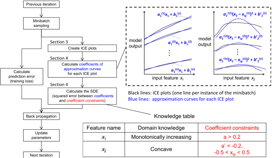
An overview of SDL is shown in Figure 1. Characteristics of the learning process of SDL are (1) to calculate not only the conventional prediction error (such as mean squared error) but also calculate Sensitivity Direction Error (SDE), and (2) to train the neural network model to minimize both the prediction error and SDE. SDE is calculated by the SDE function, which returns the squared error between coefficients of the approximation curve for each ICE plot and coefficient constraints which represent domain knowledge. Since low SDE means that approximate shapes of each ICE plot matches domain knowledge, the generalization performance of the low SDE model expects to be superior to that of high SDE models if prediction errors of the models are the same level. In this paper, five types of relationships (Increase, Decrease, Convex, Concave, and Negligible), which represent domain knowledge, are described. Furthermore, it can be applicable to other relationships where domain knowledge can be expressed as coefficient constraints. We call these approximate relationships sensitivity directions and these domain knowledge knowledge table, which consists of sensitivity directions and values of coefficient constraints for each feature.
We ran two experiments. In experiment 1, it was confirmed that SDL actually learned neural network models with five types of user-specified relationships using the generated dataset. In experiment 2, using three actual datasets, it was confirmed that SDL has the potential to achieve the same or better prediction performances than five kinds of baseline machine learning algorithms (three non-shape-constrained and two shape-constrained algorithms).
| Update |
|---|
| parameters |
| Next iteration |
| Target relationship | ||
|---|---|---|
| Approach | Only monotonicity | Including convexity |
| Model architecture | MN [1998], MNN [2010], UMNN [2019], etc. | ELN [2016], ICNN [2017], DLN [2018], etc. |
| Learning process | PWL [2019] | This paper |
2 RelatedWork
The first algorithm which can impose hard monotonicity constraints is to positively or negatively limit the neural network weights using single-layer neural networks [Archer and Wang, 1993]. Monotonic Networks (MN) [Sill, 1998] and Monotone Neural Networks (MNN) [Daniels and Velikova, 2010] extended to using multiple layers. Unconstrained Monotonic Neural Networks (UMNN) [Wehenkel and Louppe, 2019] used monotonic activation functions. In addition, Input Convex Neural Networks (ICNN) [Amos et al., 2017] can impose hard convexity constraints by using unique architectures such as convex activation functions and passthrough layers, and it was extended to the ShapeConstrained Neural Network (SCNN) [Gupta et al., 2018] which uses ReLU activation functions instead of convex activation functions. Ensemble lattice networks (ELN) [Canini et al., 2016] and Deep lattice networks (DLN) [You et al., 2017] can impose hard monotonicity and also convexity [Gupta et al., 2018] constraints by using unique architectures such as a linear calibrator and an ensemble of lattices. These algorithms have characteristics that can impose hard monotonicity and/or convexity constraints by changing the model architecture. On the other hand, soft monotonicity constraint algorithms that change the learning process were also proposed. One of these algorithms uses a point-wise loss (PWL) function [Gupta et al., 2019] which returns the error between the partial derivatives of the output of the model with respect to each input feature and constraints for the sign of each partial derivative.
As mentioned in Section 1, we consider that (1) convexity constraints should also be able to be imposed, and (2) changing the learning process has the advantage that it can be used universally for the existing neural network architecture. However as far as we know, there are no studies that satisfy both factors. Therefore, we believe that our research contributes to the field as shown in Table 1.
3 Preliminaries
Our algorithm (SDL) uses Individual Conditional Expectation (ICE) plots. This section will briefly discuss ICE plots.
For ease of understanding, we will start with the Partial Dependence (PD) plot which is the previous study of the ICE plot. The PD plot is one of the model-agnostic methods that visualizes the relationship between the output of the model and one input feature based on Equation 1.
Where xk is the value of one input feature to visualize the relationship, and ˆ f is the trained model. X(i) c is the 1-d vector of all input features of the model without xk, and n is the sample number of instances in the given dataset and ¯ f (xk) is the partial dependence, which means averaging outputs of the model for each instance in the given dataset while fixing the value of xk. Therefore, by checking PD plots, the approximate shape of the relationship between the output of the model and target input feature can be evaluated.
The ICE plot can visualize the relationships between xk and each instance of ˆ f (xk , X(i) c ). Compared to checking PD plots, checking ICE plots is especially important when approximate shapes of each ICE plot are very different.
4 Sensitivity Direction Learning
Our proposal can be divided into four parts:
- Variable definition of coefficient constraints that are required to evaluate whether approximate shapes of each ICE plot match user-specified relationships.
- The estimation algorithm about coefficients of the approximation curve for each ICE plot of the model.
- The SDE function which returns the squared error between coefficients of the approximation curve and coefficient constraints which represent domain knowledge.
- The learning process of SDL during one iteration.
4.1 Variable Definition of Coefficient Constraints
Coefficient constraints mean such as upper and lower limits for coefficients of the approximation curve for each ICE plot. We define variables of coefficient constraints for judging the following five types of sensitivity directions. In addition, the following definition process can be applicable to other kinds of sensitivity directions.
Monotonically Increasing
Increase indicates that as the input feature value x increases, the output value y also increases. To judge for Increase, the required constraint variable is the lower limit amin of the inclination a of the approximate straight line y ≈ ax.
Monotonically Decreasing
Decrease is the opposite of Increase, so that the required constraint variable is the upper limit amax.
Convex
Convex indicates that the initial behavior is Decrease, and it changes to Increase in the middle. To judge for Convex, it is necessary to know the inclination a′ of the approximate straight line dy/dx ≈ a′x, and the x coordinate of the inflection point xip. Therefore, required constraint variables are lower limit a′min of inclination a′ and upper and lower the limits (xipmax , xipmin ) of xip.
Concave
Concave is the opposite of Convex, so required constraint variables are the upper limit a′max of inclination a′ and upper and lower limits (xipmax , xipmin ) of xip.
Negligible
Negligible indicates that the absolute value of the inclination is very small, so that required constraint variables are upper and lower limits (amax, amin).
Summarizing the above arguments, required constraint variables are following: (1) amin, (2) amax, (3) a′min , (4) a′max , (5) xipmin , and (6) xipmax . We also define the sensitivity direction type tsd such as Increase, Decrease, Convex, Concave, and Negligible.
4.2 Estimation Algorithm for Constraint Variables
This subsection presents an algorithm for estimating the three coefficients (a, a′ , xip) from each ICE plot.
Putting it simply, this algorithm applies single regression analysis on ICE plots as follows:
Where, xk,j is one of arbitrary m values of xk for drawing ICE plots, and Xk is the 1-d vector that is composed of each xk,j (Xk = {xk,1, xk,2, · · · , xk,m}). Likewise, ˆ F (Xk, X(i) c ) is the 1-d vector composed of each ˆ f (xk,j , X(i) c ) and ˆ F ′ (Xk, X(i) c ) is the 1-d vector composed of each of ˆ f ′ (xk,j , X(i) c ). ˆ f ′ is the differential function of the ˆ f by xk. Outputs of the estimation algorithm are three matrices (Ak, A′ k, and Xipk ) shown in ATk = {a(1) k , a(2) k , · · · , a(n) k }, A′Tk = {a′(1) k , a′(2) k , · · · , a′(n) k }, and XT ipk = {x(1) ipk , x(2) ipk , · · · , x(n) ipk }.
Algorithm 1 calcSDE
Input: Ak, A′ k, Xipk
Input: Nk : [tsd, amax, amin, a′max, a′min, xipmax , xipmin ] Output: esdk # SDE of feature k
- 1: if tsd is Increase or Decrease or Negligible then
- 2: esdk ←calcDev(Ak, amax, amin)
- 3: else if tsd is Convex or Concave then
- 4: esdk ←calcDev(A′k , a′max, a′min)
- 5: esdk ←esdk + calcDev(Xipk , xipmax , xipmin )
- 6: else
- 7: esdk ←0.0
- 8: end if
Algorithm 2 calcDev
Input: X, xmax, xmin
Output: d # Constraint violation
- 1: d←0.0
- 2: for i = 1 : n do
- 3: x←X[i]
- 4: d←d + {MAX(x, xmax) -xmax}2 # Violating a upper constraint
- 5: d←d + {xmin -MIN(x, xmin)}2 # Violating a lower constraint
- 6: end for
- 7: d←d/n
4.3 SDE Function
The SDE function returns the squared error between coefficients (Ak, A′ k, and Xipk ) and coefficient constraints Nk (Nk = {tsd, amax, amin, a′max , a′min , xipmax , xipmin }). The algorithm of SDE function is shown in Algorithm 1. Where, esdk is the value of SDE of the feature k. esdk is calculated by the calcDev function according to the sensitivity direction type tsd. The calcDev function, as shown in Algorithm 2, calculates the constraint violation d by using the input 1-d vector X and upper and lower limits (xmax, xmin). for each element x in X. Therefore, a high esdk indicates that the relationship between the input feature k and the output of the model is differ from the user-specified relationship.
4.4 Sensitivity Direction Learning Algorithm
We will explain how SDL works in one iteration during the neural network training as shown in Algorithm 3. Where, the training dataset DT consists of l input features and one target, and N is the matrix composed of each Nk (N T = {N1,N2, · · · ,Nl}). Mixing ratio r is the hyperparameter used to adjust the priority of SDE (esd) over the prediction error (ep), and Dx consists of all input features extracted from the minibatch, and the rest is the output vector Dy. L is the conventional loss function such as the mean squared error function. ˆ fNN is the neural network model, and Xc is the matrix composed of each X(i) c (XTc = {X(1) c ,X(2) c , · · · ,X(n) c }).
In each iteration, SDL calculates the prediction error (ep) between ˆ fNN(Dx) and Dy, and also calculates SDE (esd).
Algorithm 3 Sensitivity Direction Learning (SDL)
Input: Training dataset DT , Knowledge table N Parameter: Mixing ratio r
- 1: for Each minibatch (Dx, Dy) sampled fromDT do
- 2: ep ←L ( ˆ fNN(Dx), Dy ) # Prediction error
- 3: esd ← 0.0
- # Intialize SDE
- 4: for k = 1 : l do
- 5: Nk ←N[k]
- 6: Xc ←Dx without k
- 7: Xk ←Aquire m samples from the domain of xk
- 8: Ak, A′ k, Xipk ←Xc, Xk and Equation 1 ∼ 4
- 9: esd ← esd + calcSDE(Ak, A′ k, Xipk , Nk)
- 10: end for
- 11: e ← ep + r · esd
- 12: Update parameters with e
- 13: end for
And next, updates parameters of the neural network to reduce e which is the sum of ep and r · esd. In the loop of each feature k, firstly SDL extracts Nk fromN and Xc fromDx, secondly extracts Xk which consists of m values from the domain of xk, and finally, SDL calculates SDE of feature k based on Algorithm 1. SDL minimizes both the prediction error and SDE, so that the neural network model with userspecified relationships can be obtained.
5 Experiments
We ran two experiments to answer the following basic research questions:
- Whether does SDL actually work to learn about the model with user-specified directions?
- Under what conditions is SDL effective in improving the generalization performance?
5.1 Experiment 1
In this experiment, we confirmed that SDL actually works to learn about the model with user-specified sensitivity directions using the generated dataset.
Dataset
In order to clearly confirm that SDL actually works to learn about the model with user-specified relationships, the dataset should be have relationships differed from user-specified relationships. Considering this requirement, we generated the dataset which consists of 200 instances and six columns as following steps: (i) the 1-d vector U is defined to be between 0.0 and 1.0 in 0.005 steps, and (ii) y is set to U, and each feature (x1 ∼ x5) is set to the sum of U and Gaussian noise (σ = 0.1).
As is clear from above steps, there are only strong correlations between each of five features (x1 ∼ x5) and the output y. Therefore it can be said that if a model is learned without shape constraints, there is very little possibility that the trained model has convexity relationships.
| Feature name | Sensitivity direction type | Coefficient constraints |
|---|---|---|
| x1 | Convex | 0.18 < a′ , -0.58 < xip < 0.58 |
| x2 | Concave | a′ < -0.75, -0.31 < xip < 0.31 |
| x3 | Increase | 0.53 < a |
| x4 | Decrease | a < -0.64 |
| x5 | Negligible | -0.08 < a < 0.08 |
| Mixing ratio | SDE (Med.) | SDE (SD) |
| 0.0 (Vanila NN) | 8.54 ∗ 103 | 4.02 ∗ 106 |
|---|---|---|
| 0.01 | 2.03 | 1.10 |
| 0.10 | 0.64 | 0.47 |
| 1.00 | 0.24 | 0.35 |
| 10.00 | 0.27 | 0.37 |
Knowledge Table
In this experiment, 10 kinds of knowledge tables are tested. In each table, five sensitivity directions are set for each and every input feature and coefficient constraints are populated with random samples from a uniform distribution over [0, 1) (only if the sensitivity direction is Negligible, from a uniform distribution over [0, 0.1)). As an example, one knowledge table is shown in Table 2.
Model Parameters
The neural network architecture and learning conditions are the same as in a Keras tutorial 1 , as an example to show the general settings. On the other hand, the number of epochs is set to 200 after checking for learning curves.
In the SDL algorithm, the mixing ratio r, which used to adjust the priority of SDE over the prediction error, is the most important hyperparameter, so that five kinds of candidates ({0.0, 0.01, 0.10, 1.0, 10.0}) are tested.
Experimental Results
Table 3 shows medians and standard deviations of SDE for the test dataset for each mixing ratio. In this experiment, 50 instances were randomly extracted from the dataset as the test dataset, and the rest instances were used as the training dataset. Each median and standard deviation were calculated from each result for 10 different knowledge tables. As can be seen from this table, when the mixing ratio is 0.0, which means learning without SDL, the median of SDE was extremely worse. Therefore, it was confirmed that the low SDE was due to the SDL. In addition, the minimummedian is 0.24 when the mixing ratio is 1.0, so that in this experiment, it is considered that the optimum mixing ratio value is around 1.0. This approach is considered to be generally applicable to the search for an appropriate mixing ratio.
1 https://www.tensorflow.org/tutorials/keras/regression/
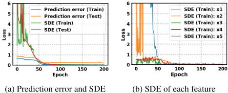
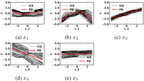
Figure 2 and 3 show the results under the conditions that the mixing ratio is set to 1.0 and the knowledge table is used shown in Table 2. Figure 2a shows learning curves of the prediction error and SDE for the training and the test dataset. From Figure 2a, it can be seen that both the prediction error and SDE approximately converged at about 50 epochs. That is, it was confirmed that the two kinds of errors did not conflict. Figure 2b shows learning curves of SDE of each input feature. From this figure, SDE of each input feature (x1 ∼ x5) all converged around 50 ∼ 100 epochs so that it can be said that SDL properly trained model with all of userspecified sensitivity directions shown in the knowledge table. Figure 3 shows PD and ICE plots of the trained model. Each ICE plot (50 black lines) corresponds to each instance of the test dataset and each PD plot (red line) is the average of black lines. From each figure, it can be said that sensitivity directions judged visually are as specified to Table 2.
Therefore, it was confirmed that SDL actually worked to learn about models with user-specified sensitivity directions.
5.2 Experiment 2
In this experiment, using three actual datasets and 5-fold cross validation, we confirmed that SDL has the potential to provide the same or better prediction performances than five kinds of baseline algorithms, such as ELN, which is the one of the state-of-the-art shape-constrained algorithm. Furthermore, we will discuss when SDL can be effective.
Dataset
Three actual datasets were chosen from the UCI Machine Learning Repository [Dua and Graff, 2017]. The first one is the Bike Sharing dataset [Fanaee-T and Gama, 2014] which consists of 731 instances and 11 features and has the characteristics that the output (count of total rental bikes (cnt)) may increase as the feeling temperature (atemp) increases. The second one is the Combined Cycle Power Plant (CCPP) dataset[T¨ufekci, 2014] which consists of 9568 instances and four features and has the characteristics that the output (energy output (ET)) may decrease as ambient temperature (AT) increases. The last one is the Bias correction of numerical prediction model temperature forecast dataset[Cho et al., 2020] which consists of 7750 instances and 23 features and has the characteristics that the output (Next Tmax) may increase as Present Tmax increases.
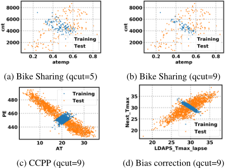
As mentioned in Section 1, the problem that SDL aims to solved is to improve the low generalization performance due to the bias in the data collection. Therefore, in these experiments, separation conditions between training and test datasets are intentionally biased. From Figure 4a and 4b, looking at the entire graph, atemp and cnt are related to strong positive correlation, but looking at the only training dataset, atemp and cnt are related to strong negative correlation. Similarly, from Figure 4c, the correlation between AT and PE is inverted, and from Figure 4d, the correlation between Next Tmax and LDAPS Tmax lapse is inverted.
Knowledge Table
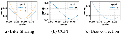
Increase is set in the sensitivity direction of atemp and temp in the Bike Sharing dataset and of Present Tmax and LDAPS Tmax lapse in the Bias correction dataset, and 15 kinds of amin candidates (between 0.0 and 1.4 in 0.1 steps) are tested. Decrease is set in the sensitivity direction of AT and RH in CCPP dataset, and 15 kinds of amax candidates (between 0.0 and -1.4 in -0.1 steps) are tested. The same amin or amax values are set for the two features in each dataset.
Model Parameters
Hyperparameters of SDL are the same as experiment 1 except the optimization function is SGD, learning rate is set to 0.1, and mixing ratio set to 1.0. To benchmark SDL performance, as baseline algorithms, three non-shape-constrained algorithms (1) ∼ (3) and two shape-constrained algorithms (4), (5) are selected: (1) Linear Regression (LR), (2) Random Forest (RF),(3) Neural Networks (NN), (4) Ensemble Lattice Networks (ELN), and (5) Constrained Linear Regression (CLR). Hyperparameters of RF are used with the default setting of scikit-learn 0.22.1[Pedregosa et al., 2011], and those of NN are the same as SDL. The basic network architecture and learning conditions of ELN are the same as in a lattice tutorial 2 . CLR means linear regression with simple weight capping by using non-negative least squares solver of scipy [Virtanen et al., 2020] so that regression coefficients of the CLR model satisfy coefficient constraints given from knowledge table. For ELN, we tune the 16 kinds of combinations of four kinds of num lattices G (3, 6, 12, 24) and lattice rank S (1, int(l/3), int(2l/3), l), and for CLR and SDL, we tune 15 kinds of amin or amax in each dataset.
Experimental Results
Table 4 shows root mean squared error (RMSE), coefficient of determination (R2) and training/inference time of each algorithm for each dataset. Each Med., SD, and Avg. were calculated from the results of 5-fold cross validation. The execution environment is Ubuntu 18.04 LTS (40 CPUs (3.00 GHz), 128 GB of Memory). In case of ELN, CLR, and SDL, tuned results, which achieved lowest median RMSE, are displayed, and tuned hyperparameters shown in rows of Param.
From Table 4 and Figure 5, RMSE and R2 of shapeconstrained algorithms were significantly better for nonshape-constrained algorithms so that shape constraints are effective when the biased dataset is used. Comparing shapeconstrained algorithms, although SDL required the most training time, SDL achieved the best RMSE and R2 in the Bike Sharing and the Bias correction datasets and the second best results in the CCPP dataset, so that it can be said that SDL has the potential to provide the same or better generalization performance than ELN and CLR.
Comparing training times of SDL and NN, since SDL required an additional training time about 12 times on average, this result means that it will take about 6 times more training time to learn one feature that is set a knowledge table than to learn a NN model. Since SDL can be particularly effective in the situation where data collection is biased, the number of the training dataset will be small in practical use. Therefore, we think the training time is unlikely to be a major problem. Nevertheless, if faster learning is needed, it is considered to use neural network techniques that make learning more efficient, or to make SDE calculation once every few iterations.
The superiority or inferiority of prediction performances between CLR and SDL tends to be similar to between LR and NN, so that it can be considered that the complexity of the task is related to these performances. In other words, if the task required an expressive power of neural networks, SDL is likely to perform better than CLR. When those performances of ELN and SDL are compared, SDL was superior in this experiment. It is considered that this is because ELN does not have hyperparameters equivalent to amin and amax (when amin or amax were set to 0.3, those performances of SDL tended to equivalent to ELN), so that it can be said that SDL has an advantage if there is domain knowledge of values of coefficient constraints.
2 https://www.tensorflow.org/lattice/tutorials/shape constraints/
| Bike Sharing (qcut=5) | Bike Sharing (qcut=9) | |||||||||||
|---|---|---|---|---|---|---|---|---|---|---|---|---|
| RMSE | R2 | Avg. time [sec] | RMSE | R2 | Avg. time [sec] | |||||||
| Algo. | Med. | SD | Med. | SD | Training | Test | Med. | SD | Med. | SD | Training | Test |
| LR | 0.934 | 0.064 | -7.757 | 1.455 | 0.001 | 0.001 | 1.284 | 0.037 | -5.672 | 0.776 | 0.001 | 0.001 |
| RF | 0.969 | 0.101 | -12.64 | 3.191 | 0.113 | 0.006 | 1.341 | 0.037 | -6.669 | 1.208 | 0.101 | 0.006 |
| NN | 0.908 | 0.088 | -5.728 | 1.951 | 1.642 | 0.001 | 1.282 | 0.046 | -4.996 | 1.474 | 1.189 | 0.001 |
| ELN | 0.591 | 0.056 | -0.098 | 0.124 | 18.65 | 1.786 | 0.621 | 0.063 | -0.176 | 0.268 | 23.51 | 2.458 |
| CLR | 0.529 | 0.062 | 0.663 | 0.107 | 0.004 | 0.001 | 0.547 | 0.047 | 0.644 | 0.066 | 0.004 | 0.001 |
| SDL | 0.510 | 0.054 | 0.676 | 0.105 | 22.45 | 0.001 | 0.515 | 0.049 | 0.708 | 0.090 | 15.72 | 0.001 |
| Param. | ELN: (G, S)=(6, 7), CLR: amin=0.3, SDL: amin=0.5 | ELN: (G, S)=(12, 7), CLR: amin=0.3, SDL: amin=0.5 | ||||||||||
| CCPP (qcut=9) | Bias correction (qcut=9) | |||||||||||
|---|---|---|---|---|---|---|---|---|---|---|---|---|
| RMSE | R2 | Avg. time [sec] | RMSE | R2 | Avg. time [sec] | |||||||
| Algo. | Med. | SD | Med. | SD | Training | Test | Med. | SD | Med. | SD | Training | Test |
| LR | 0.991 | 0.019 | -69.68 | 8.015 | 0.001 | 0.001 | 1.767 | 0.032 | -3.473 | 0.087 | 0.001 | 0.001 |
| RF | 1.149 | 0.061 | -26.00 | 10.97 | 0.252 | 0.019 | 1.483 | 0.023 | -5.894 | 0.379 | 0.780 | 0.019 |
| NN | 1.369 | 0.063 | -9.397 | 1.653 | 11.04 | 0.003 | 1.481 | 0.046 | -5.589 | 0.377 | 11.03 | 0.003 |
| ELN | 0.862 | 0.034 | -19.97 | 14.21 | 74.19 | 1.378 | 1.019 | 0.022 | -5.417 | 0.515 | 56.41 | 1.776 |
| CLR | 0.328 | 0.008 | 0.894 | 0.003 | 0.004 | 0.001 | 0.794 | 0.018 | -0.058 | 0.137 | 0.007 | 0.001 |
| SDL | 0.414 | 0.031 | 0.817 | 0.037 | 141.59 | 0.003 | 0.759 | 0.024 | 0.079 | 0.087 | 119.01 | 0.003 |
| Param. | ELN: (G, S)=(12, 4), CLR: amax=0.5, SDL: amax=0.7 | ELN: (G, S)=(3, 15), CLR: amin=0.9, SDL: amin=1.1 | ||||||||||
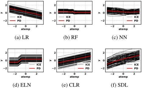
Figure 6 shows the change in RMSE for different values of amin or amax in each dataset. As can be seen from figures, if there is no knowledge of optimal values of amin or amax, it is better to set smaller values, such as 0.2, because too large values may adversely affect the performance. Alternatively, it is effective to tune values as in this experiment.
6 Conclusion
This paper proposes Sensitivity Direction Learning (SDL) for learning about a neural network model with user-specified relationships by imposing soft shape constraints which represent domain knowledge. We believe that our research contributes to the field of learning about a neural network model by imposing soft shape constraints. From experimental results, it is considered that SDL can be highly applicable if the following conditions are met: (1) you have domain knowledge about sensitivity directions and especially about values of coefficient constraints, and (2) you expect an expressive power of neural networks. As an example of use cases, we are using SDL to learn about a model for the equipment which handles complex physical phenomena such as combustion, chemical process, etc, and using the trained model for optimization of operating parameters.
Acknowledgements
We would like to thank Satoshi Hara (Osaka University) for his kind guidance on points to keep in mind when writing and submitting papers. And we would like to thank my colleagues, especially Leandro Hideo Iha, for helpful comments.
@inproceedings{ijcai2021p422,
  title     = {Sensitivity Direction Learning with Neural Networks Using Domain Knowledge as Soft Shape Constraints},
  author    = {Wakasugi, Kazuyuki},
  booktitle = {Proceedings of the Thirtieth International Joint Conference on
               Artificial Intelligence, {IJCAI-21}},
  publisher = {International Joint Conferences on Artificial Intelligence Organization},
  editor    = {Zhi-Hua Zhou},
  pages     = {3067--3074},
  year      = {2021},
  month     = {8},
  note      = {Main Track},
  doi       = {10.24963/ijcai.2021/422},
  url       = {https://doi.org/10.24963/ijcai.2021/422},
}
TY - CPAPER TI - Sensitivity Direction Learning with Neural Networks Using Domain Knowledge as Soft Shape Constraints AU - Wakasugi, Kazuyuki T2 - Proceedings of the Thirtieth International Joint Conference on Artificial Intelligence, IJCAI-21 PB - International Joint Conferences on Artificial Intelligence Organization PY - 2021 SP - 3067 EP - 3074 DO - 10.24963/ijcai.2021/422 UR - https://doi.org/10.24963/ijcai.2021/422 ER -Copied
Machine-readable versions of this paper, for tools and AI agents:





