
Minimization of Limit-Average Automata
Proceedings of the Thirtieth International Joint Conference on Artificial Intelligence. Main Track. Pages 2819-2825.
https://doi.org/10.24963/ijcai.2021/388
Keywords
- Agent-based and Multi-agent Systems: Formal Verification, Validation and Synthesis
- Machine Learning: Active Learning
- Multidisciplinary Topics and Applications: Validation and Verification
Abstract
LimAvg-automata are weighted automata over infinite words that aggregate weights along runs with the limit-average value function.
In this paper, we study the minimization problem for (deterministic) LimAvg-automata.
Our main contribution is an equivalence relation on words characterizing LimAvg-automata, i.e.,
the equivalence classes of this relation correspond to states of an equivalent LimAvg-automaton.
In contrast to relations characterizing DFA, our relation depends not only on the function defined by the target automaton, but also on its structure.
We show two applications of this relation.
First, we present a minimization algorithm for LimAvg-automata, which returns a minimal LimAvg-automaton among those equivalent and structurally similar to the input one.
Second, we present an extension of Angluin's L^*-algorithm with syntactic queries, which learns in polynomial time a LimAvg-automaton equivalent to the target one.
- [Alur et al., 2017] Rajeev Alur, Konstantinos Mamouras, and Caleb Stanford. Automata-based stream processing. In ICALP 2017, volume 80 of LIPIcs, pages 112:1-112:15. Schloss Dagstuhl -Leibniz-Zentrum für Informatik, 2017.
- [Angluin and Fisman, 2016] Dana Angluin and Dana Fis- man. Learning regular omega languages. Theor. Comput. Sci., 650:57-72, 2016.
- [Angluin et al., 2018] Dana Angluin, Udi Boker, and Dana Fisman. Families of DFAs as acceptors of ω-regular lan- guages. LMCS, 14(1), 2018.
- [Angluin, 1987] Dana Angluin. Learning regular sets from queries and counterexamples. Information and computa- tion, 75(2):87-106, 1987.
- [Beimel et al., 1999] Amos Beimel, Francesco Bergadano, Nader Bshouty, Eyal Kushilevitz, and Stefano Varricchio. Learning functions represented as multiplicity automata. Journal of the ACM, 47, 10 1999.
- [Brainerd, 1968] Walter S Brainerd. The minimalization of tree automata. Information and Control, 13(5):484-491, 1968.
- [Calbrix et al., 1993] Hugues Calbrix, Maurice Nivat, and Andreas Podelski. Ultimately periodic words of rational w-languages. In MFPS 1993, pages 554-566, 1993.
- [Cerný et al., 2013] Pavol Cerný, Thomas A. Henzinger, and Arjun Radhakrishna. Quantitative abstraction refinement. In POPL 2013, pages 115-128. ACM, 2013.
- [Chatterjee et al., 2010] Krishnendu Chatterjee, Laurent Doyen, and Thomas A. Henzinger. Quantitative lan- guages. ACM Trans. Comput. Log., 11(4):23:1-23:38, 2010.
- [Cormen et al., 2009] Thomas H Cormen, Charles E Leiser- son, Ronald L Rivest, and Clifford Stein. Introduction to algorithms. MIT press, 2009.
- [Henzinger and Otop, 2017] Thomas A Henzinger and Jan Otop. Model measuring for discrete and hybrid systems. Nonlinear Analysis: Hybrid Systems, 23:166-190, 2017.
- [Maler and Staiger, 1997] Oded Maler and Ludwig Staiger. On syntactic congruences for omega-languages. Theor. Comput. Sci., 183(1):93-112, 1997.
- [Michaliszyn and Otop, 2020] Jakub Michaliszyn and Jan Otop. Learning deterministic automata on infinite words. In ECAI 2020 -24th European Conference on Artificial Intelligence, volume 325 of Frontiers in Artificial Intel- ligence and Applications, pages 2370-2377. IOS Press, 2020.
- [Miekisz, 2008] Jacek Miekisz. Evolutionary game theory and population dynamics. In Multiscale problems in the life sciences, pages 269-316. Springer, 2008.
- [Nerode, 1958] Anil Nerode. Linear automaton transforma- tions. Proceedings of the American Mathematical Society, 9(4):541-544, 1958.
- [Rich, 2008] Elaine Rich. Automata, computability and com- plexity: theory and applications. Pearson Prentice Hall Upper Saddle River, 2008.
- [Schewe, 2010] Sven Schewe. Beyond hyper- minimisation-minimising DBAs and DPAs is NP- complete. In FSTTCS 2010, pages 400-411, 2010.
References were extracted automatically from the PDF and may contain errors.
Full text extracted automatically from the PDF; figures, tables and equations may differ. The PDF is the version of record.
1 Introduction
Automata have a wide range of AI-related applications, such as natural language processing, verification, compiler construction and others [Rich, 2008]. In many of these applications, the size of the constructed automaton has a far greater impact on performance than the time spent on construction of the automaton. Therefore, it is desirable to develop tools that reduce the number of automata states.
There are various minimization algorithms for (deterministic) finite-state automata over finite words [Nerode, 1958], deterministic weighted automata over finite words [Beimel et al., 1999] or deterministic finite tree automata [Brainerd, 1968]. They are typically based on the right congruence relation of a given language, which characterises the minimal automaton, i.e., the minimal automaton can be constructed over the equivalence classes of the right congruence relation. This approach does not extend to infinite-word automata as the right congruence relation does not characterize deterministic B¨uchi automata [Maler and Staiger, 1997]. Furthermore, the minimization problem for deterministic B¨uchi automata is NP-complete [Schewe, 2010], thus establishing a simple relation characterizing languages of these automata is elusive.
In this paper, we study the minimization problem for (deterministic) LIMAVG-automata [Chatterjee et al., 2010], which are weighted automata over infinite words. In these automata, each transition has a rational weight. The run over an infinite word w produces an infinite sequence of weights and the value of w returned by the automaton is the limit of the partial averages of this sequence of weights.
While typical infinite-word automata (e.g. B¨uchi automata) express properties regarding finite or infinite occurrences of specified events, LIMAVG-automata return more precise answers regarding the long-run frequency of specified events. This makes LIMAVG-automata an attractive specification formalism capable of expressing quantitative system properties [Cern´y et al., 2013; Henzinger and Otop, 2017], stream properties [Alur et al., 2017], or even population dynamics in evolutionary games [Miekisz, 2008]. In all these applications, the size of the automaton has a far greater impact on the performance than the time spent on its construction. Therefore, implementations involving LIMAVG-automata would greatly benefit from employing minimization of these automata. Yet, to the best of our knowledge, there is no work on the minimization of LIMAVG-automata.
1.1 Plan and Contributions
This paper is the first work on minimization of LIMAVGautomata. We begin with basic definitions (Section 2) followed by the discussion on various sources of difficulty in minimization of LIMAVG-automata (Section 3). Next, we present our main contributions.
In Section 4, for a given LIMAVG-automaton T , we define the relation ∼=T on words that characterizes T , i.e., we construct a LIMAVG-automaton equivalent to T , whose states are equivalence classes of ∼=T . Unlike the right-congruence relation, which is defined for the language of an automaton, the relation ∼=T depends on the structure of T . Therefore, the automaton obtained by minimization with respect to ∼=T is not only semantically equivalent to T , but also has similar structural properties as T . The latter property facilitates explainability of the minimized automaton.
Then, we show two applications of ∼=T . In Section 5, we employ∼=T tominimize an LIMAVG-automata in polynomial time. In Section 6, we propose an active learning framework for LIMAVG-automata and develop an active learning algorithm LIMAVG-automata utilizing ∼=T .
1.2 RelatedWork
As mentioned above, this is the first paper on minimizing LIMAVG-automata. The most closely-related work to this is [Michaliszyn and Otop, 2020], where an algorithm for learning deterministic B¨uchi automata is presented. The common ingredient is the syntactic approach: the learning algorithm of [Michaliszyn and Otop, 2020] is based on queries regarding a syntactic function called loop-index. This is similar in principle to the algorithm we present in Section 6. However, the key property of deterministic B¨uchi automata that makes the algorithm of [Michaliszyn and Otop, 2020] work is that a word that does not belong to the language is a proof that all the states it visits infinitely often are non-accepting. We discuss in Section 3 that this kind of argument fails in the LIMAVG case, and thus the algorithm of [Michaliszyn and Otop, 2020] cannot be simply adapted.
For other types of infinite-word automata, it has been shown that deciding, given k and a Deterministic B¨uchi automaton (DBA) A, whether A admits a language-equivalent DBAA′ of at most k states, is NP-complete [Schewe, 2010]. It follows that there is no polynomial-time minimization algorithm for DBA, and no learning algorithm for DBA that returns a minimal-size DBA. To bypass this hardness, various techniques have been employed. To learn an ω-language L, [Calbrix et al., 1993] considers learning languages of finite words of the form L$ = {u$v | uvω ∈ L}, where the word u$v is intended to represent the word uvω . However, the size of the constructed deterministic finite automaton can be exponential in the size of the minimal DBA. In [Calbrix et al., 1993], it has been shown that ω-regular languages that can be recognized with a DBA and with a deterministic coB¨uchi automaton can be learned in polynomial time. Another approach [Angluin et al., 2018] is to learn DBA into some different formalism, called Families of DFA (FDFA) [Angluin and Fisman, 2016]. Such FDFA can be transformed to deterministic parity automata, but with an exponential blowup [Angluin et al., 2018].
2 Preliminaries
A word w over a finite alphabet Σ of letters is a finite or infinite sequence of letters. An ultimately periodic word is a word of the form wvω . The sets of all finite and infinite words over Σ by denoted by Σ∗ and Σω respectively.
For any sequence w, including words, we define w[i] as the i-th element (letter) of w, and we define w[i, j] as the subsequence (subword) w[i]w[i+1] . . . w[j] of w. We assume that sequences start with 0 index.
Deterministic finite-state and ω-automata. A deterministic finite-state automaton (DFA) is a tuple 〈Σ,Q, q0, F, δ〉 consisting of the alphabet Σ, a finite set of states Q, the initial state q0 ∈ Q, a subset F ⊆ Q of accepting states, and a transition function δ : Q × Σ → Q.
An (deterministic) ω-automaton is a DFA such that all states are accepting. DFA and deterministic ω-automata differ in semantics. In this paper, we consider only deterministic automata and hence we omit the word "deterministic".
The size of an automaton A, denoted by |A|, is its number of states.
Semantics of automata. We extend δ to ˆ δ : Q × Σ∗ → Q inductively: for each q, we set ˆ δ(q, ϵ) = q, and for all w ∈ Σ∗ , a ∈ Σ, we set ˆ δ(q,wa) = δ(ˆ δ(q,w), a). Given a finite word w, the run π of a DFA A on w is the sequence of states ˆ δ(q0, ϵ)ˆ δ(q0, w[0])ˆ δ(q0,w[0, 1]) . . . . The run is accepting if the last state belongs to F. The language of A, dented by L(A), is the set of words having an accepting run.
An ω-automaton processes infinite words and a run over an infinite word is defined as for DFA.
Deterministic LIMAVG-automata. A (deterministic) LIMAVG-automaton A is a pair 〈B,wt〉 such that B is an ω-automaton and wt : Q×Σ → Q is a labeling of transitions of A with rationals, called weights. As for ω-automata, we consider only deterministic LIMAVG-automata and hence we omit the word "deterministic".
A run π of a LIMAVG-automaton A on a word w is the run of B on w. Every run π of A on an infinite word w defines a sequence of weights wt(π) of successive transitions of A, i.e., wt(π)[i] = wt(π[i - 1], w[i]). The value of the run π is then defined as LIMAVG(π) = limsupk→∞AVG(π[0, k]), where for finite runs π we have AVG(π) = SUM(π)/|π|, where SUM if the sum of the weights of the run. The value of a word w assigned by the automaton A, denoted by A(w), is the value of the run of A on w.
A LIMAVG-automaton A defines the function L(A): Σω → R such that L(A)(w) = A(w). We say that LIMAVG-automata A1,A2 are equivalent if and only if they define the same function, i.e., L(A1) = L(A2). Checking equivalence can be done in polynomial time [Chatterjee et al., 2010], and the if two deterministic automata are not equivalent, then there is an ultimately-periodic word wvω , where |w|, |v| are of polynomial length, distinguishing them.
ω-generators and factorizations. A run of an ωautomaton on an ultimately periodic word is an ultimately periodic sequence, but the cycle in the run can start in a different position than the cycle in the word. We define factorization of a given word to capture that.
An ω-generator is a pair (w, v) ∈ Σ∗ × (Σ∗ \ {ϵ}). For an ω-generator (w, v), we say that (u0, u1) is a factorization of (w, v) with respect to an ω-automaton A if and only if (i) wvω = u0uω1 , and (ii) there is a number c > 0 such that in the run π on wvω for all i > |u0| we have π[i] = π[i + c].
Note that in the definition of a factorization we do not require minimality and hence every ω-generator has infinitely many factorizations. Furthermore, if (u0, u1) is a factorization w.r.t. A, the automaton A does not necessarily have a cycle over u1; it can be over some power uk1 .
3 Challenges
We discuss various sources of difficulty that appear in attempting to minimize LIMAVG-automata.
3.1 The Right Congruence Relation Is Insufficient
The minimization of DFA is based on the right congruence relation ∼L⊆ Σ∗ × Σ∗ of L. For v, u ∈ Σ∗ we have u ∼L v if and only if for all w ∈ Σ∗ it holds that uv ∈ L ⇐⇒ vw ∈ L. The Myhill-Nerode theorem [Nerode, 1958] states that L is regular exactly when ∼L has finitely many equivalence classes. Moreover, the relation ∼L defines the minimal DFA recognizing L; equivalence classes of ∼L correspond to states of the minimal DFA, while transitions can be defined in a natural way. The Myhill-Nerode theorem has its counterparts for various types of automata such as tree automata [Brainerd, 1968] or weighted automata [Beimel et al., 1999].
We define the counterpart of ∼L for LIMAVG-automata. For a LIMAVG-automaton T we define ∼T over Σ∗ in the following way: for all u, v ∈ Σ∗ we have u ∼T v if and only if for all w ∈ Σω it holds that T (uw) = T (vw).
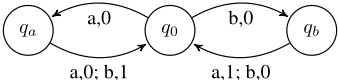
However, the Myhill-Nerode theorem does not hold for LIMAVG-automata. Consider the automaton Aab presented in Figure 1 with q0 being the initial state. It has two equivalence classes of ∼T : the class [ϵ]∼T containing all the words with even length and [a]∼T containing all the remaining words. To see that the classes are different, consider words u of odd length and v of even length. Then Aab(u(aabb)ω ) = 12 and Aab(v(aabb)ω ) = 0. All the words of even length are in the same equivalence class because after reading them, the automaton is in the state q0. The most interesting part is that all odd length words are in the same equivalence class: this is because after reading such a word, the automaton can be in qa or qb, but, after reading any letter, it will be in q0. Since LIMAVG does not depend on finite prefixes, for any v, v′ of odd length and w ∈ Σω we have Aab(vw) = Aab(v′w).
Observe that there is no equivalent LIMAVG-automaton based on these equivalence classes. Such an automaton would require two states, q′0 and q′a , such that δ(q′0 , a) = δ(q′0 , b) = q′a and δ(q′a , a) = δ(q′a , b) = q′0 . To define the weights wt, observe that the following equations need to be satisfied:
By adding top two equations and subtracting the bottom two, we obtain 0 = -2, a contradiction.
In Section 4 we present a relation refining the right congruence relation characterizing LIMAVG-automata.
3.2 Minimal Automata Are Not Unique
We present two examples of ambiguity, which we generalise later on.
Consider automata Aa, Ab resulting from changing the initial state in the automaton Aab from Figure 1 to qa and qb respectively. Observe that for every infinite word w, the runs in Aa and Ab over w differ only in the first transition to q0, while the whole infinite suffix is the same. Therefore, the word w has the same value in both automata and hence Aa and Ab are equivalent.

Consider automata Aab,L and Aab,R defined as an extension of Aab in the following way. Both automata have an additional state s0, which is initial and has a self-loop over a of the weight 0. The automaton Aab,L moves with the weight 0 to qa from Aab, while Aab,R moves on b with the weight 0 to qa from Aab. Observe that both automata are equivalent
More generally, in any LIMAVG-automaton T , changing the initial state q0 to another state q equivalent w.r.t. the right congruence (i.e., the state q such that for every u if ˆ δ(q0, u) = q, then ϵ ∼T u) preserves equivalence of automata. Furthermore, it follows that transitions between strongly-connected components are not unique as long as the target states are equivalent w.r.t. the right congruence.
3.3 Weights Are Ambiguous
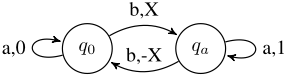
Now, we discuss why the weights in LIMAVG-automata are not uniquely defined. First, consider automata AX,Y from Fig. 2. These automata are minimal and all pairwise equivalent, since LIMAVG does not depend on finite prefixes.
We further argue that even the values of edges that are on some cycles are not uniquely defined. Consider any X ∈ Q and the automaton A±X presented in Figure 3. Then, this automaton is equivalent to A±0 . This is because for any word w, the difference between the partial sum for any prefix of the runs of A±X and A±0 on w is bounded by X, and thus the limits are the same. The same thing can happen in virtually every automaton with more than one state: if we take an automaton A, a state q and a number X ∈ Q, and define AX as a copy of A, expect that all the incoming edges (except for self-loops) to q have weights increased by X, and all the outgoing edges (except for self-loops) from q have weights decreased by X, then A and AX are equivalent. We call this "pushing weights". It demonstrates that every single weight of an automaton, except self-loops, can be set arbitrarily.
A more general issue regarding weights is called nonlocality. In the deterministic B¨uchi automata case, a word that does not belong to the language is a witness that all the states it visits infinitely often are rejecting. This is the fundamental idea of [Michaliszyn and Otop, 2020]. In the LIMAVG case, a single ultimately-periodic word only defines the average value of its ultimately-periodic cycle, but the values of the particular edges can be "pushed", as showed above. Thus, computing weights for the automaton has to be done globally.
4 Characterization of Automata
In this section we introduce a relation ∼=T on words, which characterizes a given LIMAVG-automaton T . This relation is an intersection of two relations: ∼T , which is a counterpart of the classical right-congruence relation (as discussed in the previous section), and ≡T , which is a syntactical relation. This in turn, can be used to construct a LIMAVGautomaton equivalent to T , whose states correspond to equivalence classes of ∼=T .
Definition 1. Given a LIMAVG-automaton T , we define the right-congruence relation ∼T , the cycle-equivalence relation ≡T and the mixed relation ∼=T on Σ∗ as follows:
izes to (uc, d) iff (vc, d) factorizes to (vc, d),
Note that ∼T , ≡T and ∼=T are equivalence relations.
Observe that relation ∼T is semantic, i.e., it depends only on the function defined by T . In particular, it is invariant under equivalence, i.e., swapping T with an equivalent LIMAVG-automaton does not change this relation. In contrast, relation ≡T depends on the structure of T , while it does not depend on weights of T . In other words, u ≡T v holds if for all words c, d ∈ Σ∗ , either from both states ˆ δT (qT 0 , uc) and ˆ δT (qT 0 , vc), the automaton T has cycles labeled by some powers of d, or from none of them.
Definition 2. For the relation ∼=T of T , we say that an ωautomaton B = 〈Σ,Q, q0, δ〉 is consistent with ∼=T if it satisfies the following conditions: (1) Q is the set of equivalence classes of ∼=T , (2) q0 = [ϵ]∼=T is the equivalence class of the empty word ϵ, and (3) for all q ∈ Q and a ∈ Σ, there exists u s.t. [u]∼=T = q such that δ(q, a) = [ua]∼=T .
A consistent automaton clearly exists. We show that it is unique and can be extended to an automaton equivalent to T .
Theorem 3. For every LIMAVG-automaton T , there exists a consistent ω-automaton B, which is (a) unique, and (b) there exists labeling wt of transitions of B with rational numbers such that the resulting LIMAVG-automaton (B,wt) is equivalent to T . Such a labeling wt can be computed in polynomial time in |T |.
The proof of (a) follows from the fact that ∼=T is a congruence. Based on this, we create B in the straightforward way. To show (b), we pick an automaton T , an equivalence class [u]∼=T and define Su as the set of states s such that if δT (qT 0 , v) = s then u ∼=T v. States Su can be contracted to a single state qS and the resulting LIMAVG-automaton Au is equivalent to T . Relations ∼=T and ∼=Au coincide. We iterate this process until we obtain a LIMAVG-automaton A∗ such that each state of A∗ corresponds to a single equivalence class of ∼=T . The automaton A∗ is equivalence to all its predecessors and in particular T and it is isomorphic to B. Therefore, the weights wt of A∗ can be transferred to B.
To compute wt, we can create in polynomial time a system of linear equations whose solution defines wt. The details can be found in the extended version of this paper.
5 Minimization Algorithm
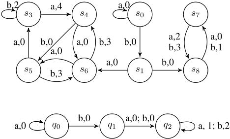
In this section we present a minimization algorithm for LIMAVG-automata. For a given LIMAVG-automaton T the presented algorithm constructs an automaton whose states are the equivalence classes of ∼=T . This automaton has at most as many states as T . However, it does not need to be minimal among all LIMAVG-automata equivalent to T . Indeed, if T has a complex structure, its cycle-equivalence is likely nontrivial. However, if it has only 0 weights, then it is equivalent to a single-state LIMAVG-automaton. Figure 4 is an example of how the algorithm works: it reduces an 8-states automaton to a 3-states automaton, while the minimal semantically equivalent automaton has 2 states.
The relation ∼=T is defined over words. This is a typical choice for such relations, and this will prove handy in the automata learning process (Section 6), where the automaton T is concealed and can be only queried. However, in this section, we assume the full access to the automaton T . In such a scenario, it is convenient to define relations on states rather than words. We present a canonical way to lift an equivalence relation from words to states.
Let ▷◁T be one of the symbols among ∼T , ≡T and ∼=T . We define the relation ▷◁Q, which is a counterpart of ▷◁T , as follows. For each state q of T , let Wq be the set of words w that lead to q, i.e., ˆ δT (qT 0 ,w) = q. For all q, s ∈ QT it holds that q ▷◁Q s if and only if for some words u ∈ Wq and v ∈ Ws we have u ▷◁T v. Observe that if u, u′ ∈ Wq (resp., Ws), then u ▷◁T u′ . Therefore, the choice of words u ∈ Wq and v ∈Ws is irrelevant.
The main step of the minimization algorithm is to compute the relation ∼=Q. Observe that for states q, s ∈ QT we have q ∼=Q s if and only if q ∼Q s and q ≡Q s. The algorithm works in two steps: first it constructs ∼Q, and then for each equivalence class of ∼Q, it refines the partition w.r.t. ≡Q. We discuss these two steps below.
Computing relation ∼Q. Consider q, s ∈ QT . To decide whether q ∼Q s, we construct the product automaton A× = T × T with the initial state (q, s) and the weight of each transition being the difference between weights of transitions in the components, i.e., for all q1, s1 ∈ T and a ∈ Σ we define wtA× ((q1, s1), a) = wtT (q1, a)-wtT (s1, a). Then, we check whether A× has a reachable cycle of non-zero sum of weights, which can be done in polynomial time [Cormen et al., 2009, Chapter 24]. If there is no such cycle, then the limitaverage of weights along every run in A× is 0, and hence for every word w, we have Tq(w) = Ts(w), i.e., the automaton T starting from q on w returns the same value as starting from s. Thus, q ∼Q s. Otherwise, the cycle of a non-zero sum of weights corresponds to a word w such that Tq(w) ̸= Ts(w) and hence q ̸∼Q s.
Imporved complexity. The above procedure can be optimized two work in O(|Q|4 |Σ|). The idea is to compute ∼Q for all pairs of states at once. We construct the automaton A× as previously, but we drop the initial state and labels of letters. We obtain a weighted graph G over vertexes QT × QT . We partition G into strongly connected components (SCCs). Next, for each SCC we check whether it has a cycle of a non-zero sum of weights [Cormen et al., 2009, Chapter 24]. We label all pairs of states (q, s) in SCCs with a non-zero sum cycle as non-∼Q-equivalent, and all pairs of states (q, s) from which non-∼Q-equivalent SCCs are reachable as non∼Q-equivalent as well. Finally, from any pair (q, s) of states, which are not labeled as non-∼Q-equivalent, only cycles of total sum 0 are reachable, and hence q ∼Q s. Careful analysis shows that the obtained complexity of this approach is dominated by the cost of finding non-zero cycles, which is quadratic in the number of states of the product automaton (and the number of such states is quadratic), resulting in the above-mentioned complexity.
Computing relation ≡Q. We say that q and s and not immediately cycle-equivalent if there is a word d such that for some words vq, vs ∈ Σ∗ that lead to q and s respectively we have (vq, d) factorizes to (vq, d), while (vs, d) does not factorize to (vs, d) (or the same with q and s swapped). Observe that q ̸≡Q s if and only if there is a word c such that ˆ δ(q, c) and ˆ δ(s, c) are not immediately cycle-equivalent. We argue that the following conditions are equivalent:
- (i) q and s are not immediately cycle-equivalent,
- (ii) there is a word u ∈ Σ∗ such that T has a cycle over some uk from q, but for every n > 0, there is no cycle over un from s (or the same with q and s swapped), and
- (iii) there is aword u ∈ Σ∗ and a state s′ ̸= s such that T has a cycle over some u from q (ˆ δ(q, u) = q), ˆ δ(s, u) = s′ , and ˆ δ(s′ , u) = s′ (or the same with q and s swapped).
The equivalence between (i) and (ii) follows from the definition. Condition (iii) clearly implies condition (ii). For the converse, consider a word d satisfying (ii). Then, d′ = dk satisfies ˆ δ(q, d′ ) = q and for all n > 0 we have ˆ δ(s, d′ ) ̸= s. Then, there are a, b > 0 such that ˆ δ(s, (d′ )a ) = ˆ δ(s, (d′ )a+b ), and hence ˆ δ(s, (d′ )ab ) = ˆ δ(s, (d′ )ab+b ). Therefore, ˆ δ(s, (d′ )ab ) = ˆ δ(s, (d′ )ab+ab ) and dkab satisfies condition (iii).
Condition (iii) can be checked in polynomial time. We can try all states as s′ . For a fixed s′ we construct the product automaton consisting of three copies of T starting from the state (q, s, s′ ) and check whether it is possible to reach the state (q, s′ , s′ ). This can be done in time O(|V |4 |Σ|).
We mark all pairs q and s that are not immediately cycleequivalent as not ≡Q-equivalent and back propagate, i.e., if q′ , s′ are such that δ(q′ , a) = q and δ(s′ , a) = s then we mark q′ and s′ as not ≡Q-equivalent. The back-propagation can be done in time O(|V |4 |Σ|).
The minimization. The intersection of ≡Q and ∼Q yields ∼=Q . We construct an automaton A = 〈Σ,Q, q0, δ,Q,wt〉 in the following way. The set Q ⊆ QT is any selector of equivalence classes of ∼=Q, and q0 is the representative of the equivalence class of qT 0 . The transition relation is defined as follows: for q ∈ Q and a ∈ Σ we define δ(q, a) as the representative from Q of the equivalence class of δT (q, a). Observe that the ω-automaton 〈Σ,Q, q0, δ,Q〉 is consistent with ∼=T . Therefore, by Theorem 3 we can compute wt : Q× Σ → Q in polynomial time such that the LIMAVG-automaton A = 〈Σ, Q, q0, δ, Q, wt〉 is equivalent with T .
Theorem 4 (Minimization w.r.t. ∼=T ). Given a LIMAVGautomaton T , we can compute in polynomial time in |T | a LIMAVG-automaton A, which is equivalent to T , and each state of A corresponds to a different equivalence class of ∼=T .
6 Learning Algorithm
We present an active learning algorithm for (deterministic) LIMAVG-automata base on L∗ -algorithm [Angluin, 1987].
We construct the relation ∼=T iteratively. We start with defining a relation ∼=TC , which is a version of the relation ∼=T parametrized by a set of ω-generators C. The relation ∼=TC approximates its non-parameterized counterpart. We show that there is a parameter C of polynomial size in T such that ∼=TC and ∼=T coincide. The learning algorithmwill learn such a C.
The equivalence classes of ∼=T can be characterized by means of the following function TLVTu . Let TLVTu (c, d) be defined as the pair (T (ucdω ), e), where e is the boolean value representing whether (uc, d) factorizes to (uc, d). It can be easily shown that for all words u, v we have TLVTu = TLVTv if and only if u ∼=T v.
A natural approach would be to consider queries regarding TLVT . Here, we show that even a simpler function suffices for learning: LVTu . Let LVTu (c, d) be defined as T (ucdω ) if (uc, d) factorizes to (uc, d), and ⊥ otherwise.
Definition 5 (Parameterized word relations). Given a LIMAVG-automaton T and a set of ω-generators C, we define the relation ∼=TC on Σω as follows: u ∼=TC v iff for all (c, d) ∈ C we have LVu(c, d) = LVv(c, d).
Observe that for a LIMAVG-automaton T and any two different equivalence classes [u]∼=T , [v]∼=T of ∼=T either there is an ultimately periodic word w witnessing that u ̸∼T v, or finite words c, d witnessing that u ̸≡T v. We can pick the word w to factorize in at least one of the words u, v. Therefore, there is C with at most |T |2 elements such that relations ∼=TC and ∼=T coincide. Furthermore, a pumping argument shows that we can pick C whose elements are of length at most |T |3 .
Lemma 6. For every LIMAVG-automaton T , there is a finite set of ω-generators C such that ∼=TC coincides with ∼=T .
An ω-automaton B = 〈Σ,Q, q0, δ〉 is partially consistent with ∼=TC if it satisfies the following conditions: (1) Q is a subset of the equivalence classes of ∼=T , (2) q0 = [ϵ]∼=T is the equivalence class of the empty word ϵ, and (3) for all q ∈ Q and a ∈ Σ, there exists u ∈ q such that δ(q, a) = [ua]∼=T .
The framework. For the remainder of this section we fix a target LIMAVG-automaton T . We consider the active learning setting, in which the learning algorithm asks queries to an oracle called the teacher. The teacher answers queries about the target automaton T , which is concealed from the learning algorithm. We consider the following types of queries:
| LV-value query | |
|---|---|
| Input | word u ∈ Σ∗ and ω-generator (c, d) |
| Output | LVTu (c, d) |
| LV-equivalence query | |
|---|---|
| Input | ω-automaton A |
| Output | Consistent if for all u, v such that ˆ δA(qA 0 , u)=ˆ δA(qA 0 , v) we have LVTu =LVTv , a counterexample otherwise |
We assume that a counterexample to an LV-equivalence query is a tuple 〈u, v, c, d〉 of words such that ˆ δA(q0, u) = ˆ δA(q0, v) and LVTu (c, d) ̸= LVTv (c, d).
The algorithm. Let T be the target automaton. The learning algorithm works in two stages. First, it learns an ωautomaton A consistent with ∼=T . Having the automaton B it finds the labeling wt such that 〈B,wt〉 is equivalent to the target automaton T . We discuss these two stages below.
Learning a consistent automaton. To learn an ωautomaton consistent with ∼=T , we adapt the L∗ - algorithm [Angluin, 1987]. The algorithm maintains two sets: a set of finite words S, called selectors, and a set of ω-generators C, called test words. It works by saturating S and C until (i) ∼=TC coincides with ∼=T , and (ii) every equivalence [u]∼=T contains exactly one word from S. The main body of the algorithm is presented as Algorithm 1, where T.LVEQUIVALENCE(A) is the LV-equivalence query.
For S,C, s ∈ S and a ∈ Σ, let δMAY S,C (s, a) = {s′ ∈ S | sa ∼=TC s′ } be the set of possible values of δ(s, a). Observe that testing the membership of δMAY S,C (s, a) can be done effectively: s′ ∈ δMAY S,C (s, a) if and only if for all (c, d) ∈ C we have T.LVVALUE(s′ , (c, d)) = T.LVVALUE(sa, (c, d)).
The procedure EXTEND(S, C, 〈u, v, c, d〉), defined in Algorithm 1, extends S,C to S′ ,C ′ via a fixed-point computation that makes sure that for every selector s ∈ S and every letter a ∈ Σ there is a selector s′ ∈ S such that sa ∼=TC′ s′ . If such a selector is not in S, then it extends S with sa. It terminates in polynomial time; |S| is bounded by the number of equivalence classes of ∼=TC′ , which is bounded by |T |.
Lemma 7. The procedure EXTEND(S,C, 〈u, v, c, d〉) works in polynomial time and returns S′ ,C ′ ,A such that A is partially consistent with ∼=TC and either S′ ⊃ S or S′ = S and δMAY S′ ,C′ ⊂ δMAY S,C .
Algorithm 1 The learning algorithm.
1: procedure LEARN-STRUCTURE(T) 2: S := {ϵ}, C := ∅ 3: A := the one state automaton 4: while true do 5: e := T.LVEQUIVALENCE(A) 6: if e = Consistent then return A 7: S, C, A := EXTEND(S, C, e) 8: procedure EXTEND(S,C, 〈u, v, c, d〉) 9: C := C ∪ {(xc, d) | x is a suffix of u or v} 10: δ = ∅, Done = ∅ 11: while S ̸=Done do 12: for all s ∈ S \Done, a ∈ Σ do 13: if there is s′ ∈ δMAY S,C (s, a) 14: then δ(s, a) = s′ 15: else S := S ∪ {sa}, δ(s, a) = sa 16: Done := Done ∪ {s} 17: return S, C, 〈Σ, S, ϵ, δ〉The algorithm LEARN-STRUCTURE(T) iterates the main loop at most polynomially many times and each iteration takes polynomial time. Therefore, it works in polynomial time. The termination condition implies that the returned automaton is consistent with ∼=T .
Learning weights. Consider an ω-automaton B consistent with ∼=T . We assign with each transition ei a variable xi corresponding to its weight. Suppose that transition e1 occurs in a cycle e1e2e3 labeled with aba and u leads to e1 cycle from q0. Then, the LV-query (u, aba) returns α, which is the mean of weights in the cycle e1e2e3. We express this with the equation: x1 + x2 + x3 = 3 · α.
Based on the structure of B, we can construct in polynomial time a maximal linearly independent system of linear equation characterizing weights of transitions e1, . . . , ek. It follows that every solution to that system gives rise to the labeling wt defined by wt(ei) = xi such that 〈B,wt〉 is equivalent to T .
Lemma 8. Given an ω-automaton B, we can compute a system of linear equations A⃗x =⃗b in polynomial time such that any solution ⃗x defines wt by wt(ei) = xi such that 〈B,wt〉 is equivalent to T . Furthermore, the matrix A is defined based only on B and the vector ⃗b is computed as the result of LV-value queries.
Linear equations over the rational numbers can be solved in polynomial time, thus we can effectively learn LIMAVGautomata:
Theorem 9. Active learning deterministic LIMAVGautomata with teacher answering LV-value queries and LV-equivalence queries can be done in time polynomial in the size of the target automaton and the size of teachers' responses.
Acknowledgments
This work was supported by the National Science Centre (NCN), Poland under grant 2017/27/B/ST6/00299.
@inproceedings{ijcai2021p388,
  title     = {Minimization of Limit-Average Automata},
  author    = {Michaliszyn, Jakub and Otop, Jan},
  booktitle = {Proceedings of the Thirtieth International Joint Conference on
               Artificial Intelligence, {IJCAI-21}},
  publisher = {International Joint Conferences on Artificial Intelligence Organization},
  editor    = {Zhi-Hua Zhou},
  pages     = {2819--2825},
  year      = {2021},
  month     = {8},
  note      = {Main Track},
  doi       = {10.24963/ijcai.2021/388},
  url       = {https://doi.org/10.24963/ijcai.2021/388},
}
TY - CPAPER TI - Minimization of Limit-Average Automata AU - Michaliszyn, Jakub AU - Otop, Jan T2 - Proceedings of the Thirtieth International Joint Conference on Artificial Intelligence, IJCAI-21 PB - International Joint Conferences on Artificial Intelligence Organization PY - 2021 SP - 2819 EP - 2825 DO - 10.24963/ijcai.2021/388 UR - https://doi.org/10.24963/ijcai.2021/388 ER -Copied
Machine-readable versions of this paper, for tools and AI agents:





