
Learning CNF Theories Using MDL and Predicate Invention
Proceedings of the Thirtieth International Joint Conference on Artificial Intelligence. Main Track. Pages 2599-2605.
https://doi.org/10.24963/ijcai.2021/358
Keywords
- Machine Learning: Relational Learning
- Constraints and SAT: Constraints and Data Mining; Constraints and Machine Learning
Abstract
We revisit the problem of learning logical theories from examples, one of the most quintessential problems in machine learning. More specifically, we develop an approach to learn CNF-formulae from satisfiability. This is a setting in which the examples correspond to partial interpretations and an example is classified as positive when it is logically consistent with the theory.
We present a novel algorithm, called Mistle -- Minimal SAT Theory Learner, for learning such theories. The distinguishing features are that 1) Mistle performs predicate invention and inverse resolution, 2) is based on the MDL principle to compress the data, and 3) combines this with frequent pattern mining to find the most interesting theories.
The experiments demonstrate that Mistle can learn CNF theories accurately and works well in tasks involving compression and classification.
- [Agrawal et al., 1996] Rakesh Agrawal, Heikki Mannila, Ramakrishnan Srikant, Hannu Toivonen, and A. Inkeri Verkamo. Fast discovery of association rules. In Ad- vances in Knowledge Discovery and Data Mining, pages 307-328. AAAI/MIT Press, 1996.
- [Biere, 2008] Armin Biere. Picosat essentials. Journal on Satisfiability, Boolean Modeling and Computation, 4(2- 4):75-97, 2008.
- [Coenen, 2003] Frans Coenen. The lucs-kdd dis- cretised/normalised arm and carm data library. https://www.csc.liv.ac.uk/ ∼ frans/KDD/Software/ LUCS-KDD-DN/DataSets/dataSets.html, 2003. [Online; accessed 30-May-2021]. Link
- [De Raedt and Dehaspe, 1997] Luc De Raedt and Luc De- haspe. Learning from satisfiability. In Proc. 9th Dutch Conference on Artificial Intelligence (NAIC), pages 303- 312, 1997.
- [De Raedt, 2008] Luc De Raedt. Logical and relational learning. Springer, 2008.
- [Dries et al., 2009] Anton Dries, Luc De Raedt, and Siegfried Nijssen. Mining predictive k-cnf expressions. IEEE Transactions on Knowledge and Data Engineering, 22(5):743-748, 2009.
- [Dua and Graff, 2017] Dheeru Dua and Casey Graff. UCI machine learning repository. http://archive.ics.uci.edu/ml, 2017. [Online; accessed 30-May-2021]. Link
- [Fischer and Vreeken, 2019] Jonas Fischer and Jilles Vreeken. Sets of robust rules, and how to find them. In Proc. Joint European Conference on Machine Learning and Knowledge Discovery in Databases (ECML PKDD), volume 11906 of LNCS, pages 38-54. Springer, 2019.
- [Fournier-Viger et al., 2016] Philippe Fournier-Viger, Jerry Chun-Wei Lin, Antonio Gomariz, Ted Gueniche, Azadeh Soltani, Zhihong Deng, and Hoang Thanh Lam. The SPMF open-source data mining library version 2. In Proc. Joint European Conference on Machine Learning and Knowledge Discovery in Databases (ECML PKDD), volume 9853 of LNCS, pages 36-40. Springer, 2016.
- [Grünwald, 2007] Peter D. Grünwald. The Minimum De- scription Length Principle, volume 1. The MIT Press, 2007.
- [Jabbour et al., 2013] Said Jabbour, Lakhdar Sais, Yakoub Salhi, and Takeaki Uno. Mining-based compression ap- proach of propositional formulae. In Proc. 22nd ACM Conference on Information & Knowledge Management (CIKM), pages 289-298, 2013.
- [Lucchese et al., 2004] Claudio Lucchese, Salvatore Or- lando, and Raffaele Perego. DCI closed: A fast and mem- ory efficient algorithm to mine frequent closed itemsets. In Proc. IEEE ICDM Workshop on Frequent Itemset Mining Implementations(FIMI), volume 126, 2004.
- [Muggleton and Buntine, 1988] Stephen Muggleton and Wray L. Buntine. Machine invention of first order predicates by inverting resolution. In Proc. 5th Interna- tional Conference on Machine Learning (ICML), pages 339-352.
- Morgan Kaufmann, 1988.
- [Muggleton and De Raedt, 1994] Stephen Muggleton and Luc De Raedt. Inductive logic programming: Theory and methods. The Journal of Logic Programming, 19/20:629- 679, 1994.
- [Muggleton et al., 2014] Stephen Muggleton, Dianhuan Lin, Niels Pahlavi, and Alireza Tamaddoni-Nezhad. Meta- interpretive learning: application to grammatical infer- ence. Machine Learning, 94(1):25-49, 2014.
- [Muggleton, 1987] Stephen Muggleton. Duce, an oracle- based approach to constructive induction. In Proc. 10th International Joint Conference on Artificial Intelligence (IJCAI), pages 287-292, 1987.
- [Smets and Vreeken, 2012] Koen Smets and Jilles Vreeken. Slim: Directly mining descriptive patterns. In Proc. 12th SIAM International Conference on Data Mining (ICDM), pages 236-247, 2012.
- [Valiant, 1984] Leslie G. Valiant. A theory of the learnable. Communications of the ACM, 27(11):1134-1142, 1984.
- [Van Leeuwen and Vreeken, 2014] Matthijs Van Leeuwen and Jilles Vreeken. Mining and using sets of patterns through compression. In Frequent Pattern Mining, pages 165-198. Springer, 2014.
- [Vreeken et al., 2011] Jilles Vreeken, Matthijs van Leeuwen, and Arno Siebes. Krimp: mining itemsets that compress. Data Mining and Knowledge Discovery, 23(1):169-214, 2011.
- [Zhao et al., 2006] Lizhuang Zhao, Mohammed J. Zaki, and Naren Ramakrishnan. Blosom: a framework for mining arbitrary boolean expressions. In Knowledge Discovery and Data Mining (KDD), pages 827-832, 2006.
References were extracted automatically from the PDF and may contain errors.
Full text extracted automatically from the PDF; figures, tables and equations may differ. The PDF is the version of record.
1 Introduction
Learning propositional logical theories from examples is one of the quintessential problems in machine learning, as it is the setting used to introduce the notion of probably approximately correct learning [Valiant, 1984]. It is also the most basic setting for inductive logic programming [Muggleton and De Raedt, 1994] and logical and relational learning [De Raedt, 2008]. Furthermore, the problem of frequent pattern mining, as introduced by Agrawal et al., can also be viewed as a logical learning problem as itemsets are logical interpretations or variable assignments.
One of the most fascinating aspects of logic learning is predicate invention [Muggleton, 1987; Muggleton and Buntine, 1988; Muggleton et al., 2014], that is, the ability to automatically introduce new predicates in the language that not only compresses the data, but also provides insights into the underlying regularities. Predicate invention has been studied almost exclusively in the context of logic program induction (using Prolog) with the early approaches of Muggleton; Muggleton and Buntine relying on the Minimum Description Length (MDL) principle [Gr¨unwald, 2007]. This form of predicate invention is also related to recent approaches for pattern and itemset mining such as KRIMP [Vreeken et al.,
2011] that identify codes to compress datasets. These approaches have been widely welcomed in the data mining literature [Smets and Vreeken, 2012; Van Leeuwen and Vreeken, 2014; Fischer and Vreeken, 2019].
We revisit these approaches and combine the above three settings: 1) As Valiant, we focus on learning CNFs 2) as Muggleton, we employ inverse resolution and MDL to invent new predicates and, 3) as KRIMP, we use frequent pattern mining to find the most interesting predicate definitions or codes. At the same time, we learn from satisfiability. This means that the examples are partial interpretations, that is, assignments of truth-values to some of the variables. An example e is then considered positive for a CNF theory T if T ∧ e ̸|= ✷, that is, the theory with the example is satisfiable [De Raedt and Dehaspe, 1997]. This differs from Valiant's setting and the typical itemset mining setting in the use of partial rather than complete interpretations (assignments to all the variables). Furthermore, it differs from Muggleton's settings in that we learn a CNF formula rather than a logic program, which are not only more general, but also have a different semantics.
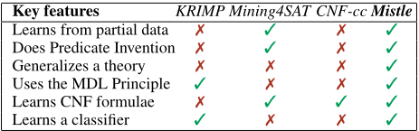
While a general framework for mining Boolean expressions has been proposed [Zhao et al., 2006], most pattern mining techniques focus on learning DNF formulae. The few approaches that focused on learning CNF theories include [Dries et al., 2009; Jabbour et al., 2013]. Dries et al. consider Valiant's k-CNF setting in their system CNF-cc and demonstrate that k-CNF formulae can be used for a wide variety of prediction tasks but do neither allow for partial interpretations nor consider predicate invention. Mining4SAT [Jabbour et al., 2013] focuses only on lossless compression and does not generalize the learned CNFs from examples.
In this paper, we introduce the Mistle algorithm for learning CNFs, which combines features from related approaches with the ability to generalize, as summarized in Table 1.
2 Background
2.1 Logic
We briefly review propositional clausal logic. Propositional variables, also called predicates here, are the basic building blocks. They can be assigned the values True or False. A literal l is a propositional variable v or its negation ¬v. A disjunction (l1 ∨ ... ∨ ln) of literals li is a clause and a conjunction (C1 ∧ ... ∧Ck) of clauses Cj is a clausal theory or a CNF formula.
An interpretation is an assignment of truth values to the propositional variables. When the mapping is available only for a subset of the variables in a domain, it is called a partial interpretation. An interpretation i is called a completion of a partial interpretation e, if it has the same variable assignments as that of e and assigns truth values to all variables in the domain. An interpretation i satisfies a clause (l1∨...∨ln) if at least one of the lj is true in i, and satisfies a clausal theory if it satisfies all the clauses in that theory. A theory T is satisfiable if there is an interpretations that satisfies it, notation T ̸|= ✷; otherwise it is unsatisfiable, notation T |= ✷. T is said to satisfy a partial interpretation, e, if and only if T ∧ e ̸|= ✷. It is also useful to know that for logical formulae α and β, α |= β if and only if α ∧ ¬β |= ✷.
2.2 Learning fromPartial Interpretations
Partial interpretations will be used as examples in this paper. Similar to concept-learning, we talk about theories that cover examples. More formally, a logical theory T covers an example e if and only if T ∧e ̸|= ✷. Here, e corresponds to a partial interpretation, that is, a conjunctive expression l1∧...∧lk stating which literals or variable assignments evaluate to T rue in the partial interpretation e. Thus, Mistle follows the learning from satisfiability [De Raedt and Dehaspe, 1997] setting.
Notice that T ∧ (l1 ∧ ... ∧ lk) |= ✷ holds if and only if T |= (¬l1 ∨ ... ∨¬lk) holds. Thus learning from satisfiability also corresponds to the learning from entailment setting that is dominant in inductive logic programming. It is only that one then learns from clauses, and that the role of the positive and negative examples is reversed. Let us also remark that when learning from satisfiability, it is in principle possible to use clausal theories as examples rather than partial interpretations, which provides added expressivity. This will work with Mistle as well except that the frequent pattern mining aspect described in Section 6.3 will no longer apply.
It is also useful to note the connection to the multi-instance learning setting [De Raedt, 2008]. If T does not cover a partial interpretation e, then it does not cover any completion of e. On the contrary, if e satisfies T , then there exists at least one completion of e that is satisfied by T .
Note that when learning from satisfiability, T1 is more general than T2 if T1 |= T2 [De Raedt and Dehaspe, 1997], which can be used to prune and partially order the search space.
2.3 Predicate Invention
Predicate Invention is the process of automatic invention of new predicates in order to represent any regularities found in the data [Muggleton, 1987; De Raedt, 2008]. This is used in Mistle and is of great importance as it allows us to compress the theory without incurring any losses.
Example 1. Let T = (a ∨ b ∨ c ∨ d ∨ e) ∧ (a ∨ b ∨ c ∨ d ∨ f) ∧ (a ∨ b ∨ c ∨ d ∨ g). Notice that all the clauses in T have a shared sub-clause a ∨ b ∨ c ∨ d. Thus, in order to compress T , we can invent a new predicate z and associate it with this sub-clause. This compresses T to a shorter theory, T ′ = (z ∨ a ∨ b ∨ c ∨ d) ∧(¬z ∨ e) ∧ (¬z ∨ f ) ∧(¬z ∨ g).
The transformation from T to T ′ is lossless in the sense that both theories cover exactly the same set of examples, that is, the same set of partial interpretations over the original variables (the variables in the dataset). Of course, when considering also the newly introduced predicate z, the space of possible interpretations becomes larger.
To understand how predicate invention is performed, it is vital to look into inverse resolution. Inverse resolution refers to inferring input clauses for resolution based upon the resolvent or the output clauses. Thus, it is an inverse of the process of resolution. In Mistle, predicate invention is performed using an inverse resolution operator called W-operator, which is delineated later in Section 4.
In the above example, the sub-clause, a∨b∨c∨d can also be thought of as a pattern occurring frequently in the theory. This consequently draws parallels to frequent itemset mining. But predicate invention offers a logical approach to find regularities in the theory. Early predicate invention systems like DUCE [Muggleton, 1987] and CIGOL [Muggleton and Buntine, 1988] even interacted with the user and allowed the user to name the newly invented predicate, keeping the theory easy to understand at all stages of the algorithm.
2.4 MDL Principle
For concept learning, one could simply construct a na¨ıve, uncompressed theory that is consistent with the data. However, as the size of such a theory explodes for larger amounts of data, compressing the theory is crucial. The MDL Principle provides a formal framework for this.
Let D be the input data, T be a theory for it, and DL be a description length measure. Then, the MDL principle states that the best theory is the one that minimises the joint description length of the theory and the data, given by
The first term denotes the description length of the theory T , the second that of the data when it is encoded using T. This definition of MDL is called the two-part MDL as it separately encodes the theory and the data [Gr¨unwald, 2007]. We define the measure DL used by Mistle in Section 5.
3 ProblemDescription
By now, we are able to formalize the problem: Given:
- a set of variables, V = {v1, v2, . . . , vm}
- a set of positive partial interpretations P
- a set of negative partial interpretations N
- a measure of description length DL
Find: a theory T ∗ over V that minimizes DL(P ∪N, T),
Thus we are looking for a theory that maximally compresses the data and classifies the examples as correctly as possible.
The first term in the right hand side aims for a simple theory. The second and third terms aim for fewer errors made by a theory in explaining the positive and negative partial interpretations, respectively. In particular, DL(P|T) measures the encoding length of the positive examples that are not satisfied in T, and DL(N|T) that of the negative examples that are satisfied in T . These terms are formally defined as:
Mistle addresses the above stated problem using 2 simple steps: 1) It initializes a theory that explains the given data. 2) It uses a set of compression operators based on inverse resolution to compress that theory as much as possible. We describe how the theory is initialized in Section 6.1 and delineate the compression operators used in the next section.
4 Compression Operators
We use four logical operators for compression: W-operator, V -operator, subsumption operator, and truncation operator. These operators are adapted from the inverse resolution operators in DUCE [Muggleton, 1987].
We use the following notation to define the operators: predicates are denoted in lowercase, like a, z, and clauses are denoted in uppercase, like A, B, or C. Furthermore, |B| denotes the number of literals in B. The invented predicate is denoted by z. We define Delta (∆) as the difference in the coverage of the input and output sets:
Operations where ∆ is not satisfiable, i.e. ∆ |= ✷, are called lossless operations.
W-operator Given two clauses A ∨ B and B ∨ C, which share B, the W- operator compresses the input by inventing a new predicate z and replacing the input with the output clauses: A∨¬z, z∨B, and C ∨¬z. The intuition behind inventing z is that z can indicate whether B is True or False. It is easy to see that W-operator is an inverse resolution operator as the input clauses can be inferred back from the output clauses by resolving on ¬z. In general,
Input
: (B ∨C1) ∧ · · · ∧ (B ∨Cn-1) ∧ (B ∨Cn)
Output : (z ∨B) ∧ (¬z ∨C1) ∧ · · · ∧ (¬z ∨Cn)
∆ :
✷
V -operator Given two clauses a∨B and B∨C, that share B, the V -operator compresses the input by replacing them with the output clauses: a ∨ B, and ¬a ∨ C. In the second input clause, B is replaced by a single literal ¬a leading to compression. Similar to the W-operator, the V -operator is also an inverse resolution operator because B ∨ C can be obtained back from the output clauses if resolved upon a. But unlike the W-operator, the V -operator is a generalization as a ∧ B ∧ ¬C represents all the cases that are covered by the input but are not covered by the output. In general,
Input
: (a ∨B) ∧ (B ∨C1) ∧ · · · ∧ (B ∨Cn-1)
Output : (a ∨B) ∧ (¬a ∨C1) ∧ · · · ∧ (¬a ∨Cn-1)
∆ :
a ∧ B ∧ ¬(C1 ∧ C2 ∧ · · · ∧ Cn-1)
Subsumption Operator The Subsumption or S-operator, is a trivial operator that discards all the specific clauses that are subsumed by another clause. For example, given two clauses, A ∨ B and B, in the input, the S-operator would only return B (follows from (A∨B) ∧B ⇐⇒ B). It is a lossless operator and results in significant compression.
Input
Output :
B
✷
∆ :
Truncation Operator The Truncation or T-operator, truncates the input clauses by retaining the shared sub-clause. For example, if there are 2 clauses, A∨B and B∨C, in the input, the T-operator would return the one clause, B. It is clearly a generalization and should only be applied when it decreases the description length, DL(D, T ).
Input
Output :
B
∆ : ¬B ∧C1 ∧C2 ∧ . . . ∧Cn
5 MDL Encoding inMistle
To use the MDL principle, we need to define how a theory is encoded in Mistle. Encoding a theory means that the full theory can be recovered from its encoded elements. Given a theory of n clauses, T = C1 ∧ · · · ∧ Cn containing m variables, we measure the description length of T in bits (based on Gr ¨unwald 2007):
where LN is the universal code for integers 1 .
LN(m) and LN(n) are the lengths of the encodings of the number m of variables and the numnber n of clauses, respectively. The sum adds, for each clause, the length log2(m) of the encoding of the clause length, and the length of encoding all its literals one by one (last term).
To encode the literals, we could have used a na¨ıve encoding of ∑|Ci| j=1 log2(2m), as there can be 2m literals in the clause (the variables and their negations). Considering previously encoded literals, we exploit the fact that if a ∈ Ci, then ¬a /∈ Ci (otherwise the clause is trivially satisfiable), and that no literal can occur more than once in a clause. This removes two possibilities of literals after sending each literal and results in a total encoding length of ∑|Ci| j=1 log2(2m-2(j-1)).
1LN(x) = log2 (2.865064) + log2 (x) + log2 (log2 (x)) + . . . (Referred from Equation 3.12 in [Gr¨unwald, 2007]).
| DL - Component | Value | Length (bits) |
|---|---|---|
| # of unique predicates # of clauses in T | 5 | LN(5) |
| 1 | LN(1) | |
| # of literals in 1st clause | 3 | log2(5) |
| 1st literal of 1st clause | c | log2(10) |
| 2nd literal of 1st clause | d | log2(8) |
| 3rd literal of 1st clause | e | log2(6) |
Algorithm 1 Mistle
Input : D = {P, N} - (Sets of partial interpretations) Output: A minimal CNF theory, T , for input data, D.
- 1: T = ¬(∨n∈N n)
- 2: while True do
- 3: T ′ = compress(T)
- 4: if DL(D, resolve(T ′ )) < DL(D, T ′ )
then T ′ = resolve(T ′ )
- 5: if T ′ == T then break else T = T ′
- 6: end while
- 7: prune(T)
- 8: return T
The error terms DL(P|T) and DL(N|T) are encoded in the same way as DL(T ). Table 2 provides an example.
6 Algorithm
As mentioned in the Section 3, the main idea behind Mistle is initializing the theory and compressing it to its minimum description length using the W, V , S, and T operators. The algorithm, as described in Algorithm 1, can be broken down into the four parts: 1) Initialize the theory [line 1]. 2) Compress the theory iteratively [line 3]. 3) Resolve the theory after each compression step, only in case this leads to a shorter description length [line 4]. 4) Prune the theory [line 7]: Remove those clauses from T that do not increase DL(D, T). Let us elucidate these components below.
6.1 Initializing the Theory
To initialize a theory, two natural starting points are a theory that precisely describes the positives, or a theory that precisely describes the negation of the negatives. In Mistle, we initialize the theory T using the latter:
This is because this theory can be directly written as a CNF by pushing the negation inside. The compression operators in Mistle can be directly applied on CNFs. But starting from the conjunction of the positives would yield a DNF and it is computationally expensive (co-NP-hard) to rewrite DNFs into CNFs, hence our choice of describing the negatives.
As T is the most specific theory, we traverse the space of all theories in a monotonic way, from the most specific to more
Algorithm 2 compress(T )
1: F =mine(T) 2: while F ̸= φ do 3: C = F.pop() 4: O = find all the operations that can be applied on C 5: op∗ = argminop∈ODL(D, (T \ C) ∪ op(C)) 6: if DL(D, (T \ C) ∪ op∗ (C)) < DL(D, T ) then 7: T = (T \ C) ∪ op∗ (C) 8: Update F w.r.t C and op∗ (C) 9: end if 10: end while 11: return Tgeneral. It keeps the search process simple, systematic and efficient. So, Mistle does not require compression operators that specialize and can only use those that generalize.
6.2 Compressing the Theory - compress(T)
Compression, described in Algorithm 2, is the most important component of Mistle. It starts with searching for a set of clauses, that contain a shared sub-clause, i.e., all the clauses in C ⊆ T that share a common set of literals. The set of shared sub-clauses is stored in F [line 1]. This step is performed using frequent itemset mining, and is explained in Section 6.3. For each C [line 3], Mistle identifies a set of all the possible operations, O, that can be applied on C to compress it [line 4]. From O, Mistle selects an operation that decreases DL(D, T ) the most w.r.t the data D = {P, N} [line 5].
6.3 Mining Frequent Itemsets - mine(T)
To compress the theory T, Mistle needs to identify a set of clauses in T that it could compress using the compression operators. This is done by mining frequent closed itemsets using the DCI Closed algorithm [Lucchese et al., 2004].
A theory can be considered as a set of clauses and a clause can be represented as a set of literals. For a frequent itemset mining system, the input is the theory, T. The transactions are the clauses that occur in T. The items and itemsets are the literals and sub-clauses, respectively. The idea is to mine frequent itemsets over all the clauses in T. Let each itemset be a sub-clause of l literals and be shared by a set of m clauses in T . Then once all the itemsets are mined, these itemsets are sorted in decreasing order based on the following criteria:
- (l -1)(m-1)-2: this is the literal reduction achieved by applying the W-operator. It is chosen as a heuristic for the possible description length reduction that can be achieved. The W-operator is chosen as it is always applicable on a mined itemset.
- l, the length of the itemset
- m, the frequency of the itemset
6.4 Resolving the Theory - resolve(T)
In Algorithm 2, lines 5 and 6 choose the operator that decreases the description length the most. While this guarantees that each step can only decrease the description length, applying many operations might actually make a previous operation compress less. In our case, a T-operation can affect the compression of an early W-operation. Recall that the Woperator can decrease the description length if the invented predicate z is used in many clauses. But, if a T-operation deletes a clause in which a predicate, invented by a previous W-operation, was used, the compression of that W-operation decreases. Eventually, this can lead to a negative compression of this W-operation: it actually increased the description length. So, we need to reverse this W-operation by resolving the output clauses upon the newly invented predicate z.
This resolving step is executed in the following manner: 1) While executing a T-operation in line 3 of Algorithm 1, all the invented predicates that were contained in the clauses deleted by T-operation are cached. 2) In line 4, for every such invented predicate, the W-operation that invented that predicate is resolved back to see if the description length decreases further. 3) In case if the description length decreases, then that W-operation is reversed in the theory.
6.5 Pruning the Theory - prune(T)
We prune the learned theory to remove any clauses whose removal decrease the description length. This pruning operation removes clauses that tend to over-fit the data and unnecessarily increase the description length. Pruning is applied as a post-processing step in Algorithm 1 and not as an operator in Algorithm 2 because of its computational cost. Indeed, the pruning operation loops over all clauses of the theory, deletes them and computes the new description length. Computing this length is costly as it requires checking whether the examples are satisfiable. Pruning as a post-processing step has also been used in other MDL-based approaches such as KRIMP.
7 Experiments
Our experimental evaluation compares Mistle against the related approaches KRIMP [Vreeken et al., 2011], Mining4SAT [Jabbour et al., 2013] and CNF-cc5 [Dries et al., 2009]. As Mining4SAT and KRIMP only use lossless operations, we consider two versions of Mistle: Mistle-Lossy is the full version of the algorithm, while Mistle-Lossless only uses lossless operations, i.e., operations in line 5 of Algorithm 2 are considered only if their ∆ is unsatisfiable. We consider the tasks of compression and classification, and the following questions:
7.1 HowAccurately CanMistle Learn a Theory?
When the actual theory is known in a domain, the accuracy can be simply defined as the percentage of all complete interpretations that are either satisfied by both theories, or not satisfied by both the theories, i.e.:
where T and T ∗ are the learned and actual theories over m variables, respectively and ω belongs to the set of all possible 2m interpretations. We use artificially generated actual theories and randomly generate data based on those theories to test the accuracy 2 . To randomly generate the actual theory T ∗ of m variables: 1) we first randomly select the number of its clauses uniformly between 2 to min(10,m). 2) For each clause ci, we choose ki uniformly between 1 to m as the number of its literals. 3) Lastly, we randomly sample ki variables without replacement and assign them a negative sign with the probability of 0.5. We then generate a dataset of P (positives) and N (negatives) based on whether a randomly sampled partial interpretation is satisfied by T ∗ . The number of clauses in the actual theory is restricted to 10 so we could sample sufficient size of P and N. To account for the cases where the size of P and N may not be balanced, Mistle learns 2 theories: T+ = Mistle(P, N) and T- = Mistle(N, P ) and selects the one which has the minimum description length.
2 Because the actual theory is usually unknown in real data.
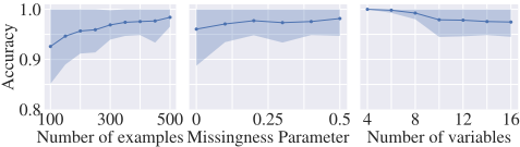
Figure 1 plots the mean accuracy for 100 generated theories and the shaded area represents the standard deviation around the mean. We individually vary 3 parameters: the number of examples, missingness parameter, and the number of variables, which have the default values of 400, 0.1 and 14 respectively. The missingness parameter is defined as the probability of not observing a literal in the data. For example, a missingness parameter of 0.1 implies that each literal in the data goes missing independently with a probability of 0.1.
The default parameters are chosen to test Mistle in a challenging and interesting setting. Using 400 examples corresponds to 2.5% of all the 214 possibilities. A missingness parameter of 0.1 tests Mistle in a non-trivial amount of noise.
It is interesting to note that in the middle plot, Mistle learns more accurate theories when the missingness is high. This is expected, as a negative partial interpretation provides more information than a complete interpretation: all completions of a negative partial interpretation are also negative. Overall, the results of this experiment validate that Mistle performs well by learning a close to perfect CNF theory in many cases.
7.2 HowMuch CanMistle Compress?
We compare Mistle against both the systems that perform compression - Mining4SAT and KRIMP. For this experiment, we use the UCI datasets [Coenen, 2003; Dua and Graff, 2017]. If a dataset has more than two classes, the most frequent class is chosen to be the positive class and the remaining classes are binned together as the negative class. Since Mining4SAT inputs a CNF theory and compresses it using operators similar to the W and S operators, we convert P and N into their respective CNFs based on Equation 6 to input to Mining4SAT: TP = ¬ (∨p ∈ P p) and TN = ¬ (∨n ∈ N n). KRIMP, on the other hand, is capable of directly taking the data as an input and compressing it. The minimum support threshold used for KRIMP and Mistle is chosen in such a way that it mines at least 10000 patterns, when so many frequent patterns exist. The compression measure used here is similar to the one used by Jabbour et al. and Vreeken et al.:
| Datasets | Minimum | Exp 2: Compression | Exp 3: Classification Accuracy | |||||
|---|---|---|---|---|---|---|---|---|
| Support Threshold | Mining4SAT | KRIMP | Mistle - Lossless | Mistle - Lossy | KRIMP | Mistle - Lossless | Mistle - Lossy | |
| Iris-17 | 1 | 7.8 | 53.2 | 75.1 | 99.3 | 99.3 | 98.7 | 100.0 |
| Iris-18 | 1 | 6.7 | 50.4 | 73.6 | 95.1 | 95.3 | 88.0 | 90.7 |
| Iris-19 | 1 | 6.7 | 50.6 | 73.6 | 94.6 | 96.0 | 94.0 | 91.3 |
| Glass | 1 | 8.8 | 28.9 | 42.0 | 84.6 | 74.8 | 71.0 | 75.7 |
| Wine | 2 | 10.7 | 21.6 | 23.9 | 95.7 | 89.9 | 60.1 | 83.7 |
| Ecoli | 1 | 37.1 | 59.9 | 79.7 | 96.2 | 93.4 | 94.6 | 78.0 |
| Hepatitis | 38 | 35.6 | 36.5 | 64.7 | 86.0 | 83.2 | 78.7 | 74.8 |
| Heart | 9 | 31.4 | 42.3 | 49.6 | 81.0 | 77.6 | 61.7 | 72.6 |
| Dermatology | 2 | 20.9 | 45.9 | 50.7 | 93.4 | 91.5 | 70.8 | 90.4 |
| Auto | 13 | 27.0 | 23.4 | 59.6 | 82.5 | 84.4 | 71.7 | 80.5 |
| HorseColic | 12 | 17.3 | 27.0 | 77.2 | 86.0 | 76.6 | 75.5 | 83.4 |
| Pima | 1 | 44.2 | 65.0 | 84.3 | 90.8 | 71.1 | 68.4 | 58.2 |
| TicTacToe | 7 | 5.4 | 37.0 | 24.9 | 99.6 | 87.7 | 65.3 | 100.0 |
| Ionoshpere | 88 | 22.7 | 17.2 | 58.7 | 93.1 | 90.3 | 64.7 | 89.5 |
| Flare | 1 | 38.7 | 61.9 | 79.2 | 99.2 | 75.9. | 47.2 | 84.0 |
| CylBands | 211 | 20.0 | 26.3 | 53.0 | 67.6 | 73.0 | 58.5 | 58.5 |
| Led | 1 | 42.8 | 75.8 | 96.3 | 98.9 | 94.9 | 79.7 | 89.1 |
| Mean | 22.6 | 42.5 | 62.7 | 90.8 | 85.6 | 73.4 | 82.4 | |
The results, plotted in Table 3, conclude that Mistle, even in the lossless case, compresses much more than Mining4SAT and KRIMP as it uses a wider set of compression operators.
As the theories we obtained using CNF-cc5 [Dries et al., 2009] were typically at least two orders of magnitude larger than those of Mistle and did not compress the data, we do not provide further details on this approach.
7.3 HowWell CanMistle Classify?
To test whether Mistle's theories are not only highly compressed but also accurate, we compare Mistle with KRIMP on a classification task, using 10 fold cross-validation on the UCI datasets. Mistle learns both T+ and T- and then uses the theory with the minimum description length w.r.t the data.
Table 3 shows that Mistle is not as accurate as KRIMP. The difference is largely due to the two datasets, Pima and CylBands. Without these two data-sets Mistle scores a mean accuracy of 85.04%, which is competitive with state-of-theart pattern mining techniques to perform classification. Note that, on the TicTacToe dataset, Mistle achieves 100% accuracy as it learns all the 8 ways (representing it in 8 clauses of 3 literals each) in which a game can be won. This experiment shows that the additional compression that Mistle obtains may come - for some datasets - with a slightly increased errorrate. However, the much more compressed theories are more explainable and provide more actionable insights. Whether this is important or not will depend on the application.
Implementation Mistle is written in Python 3.7 and uses SPMF library [Fournier-Viger et al., 2016] for closed frequent itemset mining and PicoSAT library [Biere, 2008] for SAT solving. Experiment 1 is run on Intel i5 (2.3Ghz; 16Gb RAM) while experiments 2 and 3 are run on Intel i7 (3.4 GHz; 16Gb RAM). For Experiment 2, the average runtime of Mining4SAT, KRIMP, Mistle-Lossless, and Mistle-Lossy is 5, 7, 28, and 5 seconds respectively. For experiment 3, the average runtime of KRIMP, Mistle-Lossless, and Mistle-Lossy is 19, 162, and 48 seconds respectively. On average, Mistle is slightly slower than KRIMP, which is implemented in C++.
8 Conclusions
We introduced the Mistle algorithm for learning CNFs, whose key features are denoted in the Table 1. The experiments using both real and artificial datasets cover a wide range of tasks and compare with related works. Mistle is best at learning small human-understandable logical theories in real domains. Our experiments demonstrate that Mistle can learn CNF theories quite accurately and learns highly compressed theories.
More generally, we show that learning CNF theories is better with regard to compression that the state-of-the-art system (KRIMP) for mining sets of itemsets which are similar to the DNF mining techniques. We hope that this work can lead to further research in the domain of CNF theory learning and predicate invention, and can be extended into first order logic.
Acknowledgements
This work has received funding from the European Research Council under the European Union's Horizon 2020 research and innovation programme (#694980 SYNTH: Synthesising Inductive Data Models) and from the Flemish Government under the "Onderzoeksprogramma Artifici¨ele Intelligentie (AI) Vlaanderen" programme. Luc is also supported by the Wallenberg AI, Autonomous Systems and Software Program (WASP) funded by the Knut and Alice Wallenberg Foundation.
@inproceedings{ijcai2021p358,
  title     = {Learning CNF Theories Using MDL and Predicate Invention},
  author    = {Jain, Arcchit and Gautrais, Clément and Kimmig, Angelika and de Raedt, Luc},
  booktitle = {Proceedings of the Thirtieth International Joint Conference on
               Artificial Intelligence, {IJCAI-21}},
  publisher = {International Joint Conferences on Artificial Intelligence Organization},
  editor    = {Zhi-Hua Zhou},
  pages     = {2599--2605},
  year      = {2021},
  month     = {8},
  note      = {Main Track},
  doi       = {10.24963/ijcai.2021/358},
  url       = {https://doi.org/10.24963/ijcai.2021/358},
}
TY - CPAPER TI - Learning CNF Theories Using MDL and Predicate Invention AU - Jain, Arcchit AU - Gautrais, Clément AU - Kimmig, Angelika AU - de Raedt, Luc T2 - Proceedings of the Thirtieth International Joint Conference on Artificial Intelligence, IJCAI-21 PB - International Joint Conferences on Artificial Intelligence Organization PY - 2021 SP - 2599 EP - 2605 DO - 10.24963/ijcai.2021/358 UR - https://doi.org/10.24963/ijcai.2021/358 ER -Copied
Machine-readable versions of this paper, for tools and AI agents:





