
Reinforcement Learning for Route Optimization with Robustness Guarantees
Proceedings of the Thirtieth International Joint Conference on Artificial Intelligence. Main Track. Pages 2592-2598.
https://doi.org/10.24963/ijcai.2021/357
Keywords
- Planning and Scheduling: Planning under Uncertainty
- Machine Learning: Deep Reinforcement Learning
- Machine Learning Applications: Applications of Reinforcement Learning
Abstract
Application of deep learning to NP-hard combinatorial optimization problems is an emerging research trend, and a number of interesting approaches have been published over the last few years. In this work we address robust optimization, which is a more complex variant where a max-min problem is to be solved. We obtain robust solutions by solving the inner minimization problem exactly and apply Reinforcement Learning to learn a heuristic for the outer problem. The minimization term in the inner objective represents an obstacle to existing RL-based approaches, as its value depends on the full solution in a non-linear manner and cannot be evaluated for partial solutions constructed by the agent over the course of each episode. We overcome this obstacle by defining the reward in terms of the one-step advantage over a baseline policy whose role can be played by any fast heuristic for the given problem. The agent is trained to maximize the total advantage, which, as we show, is equivalent to the original objective. We validate our approach by solving min-max versions of standard benchmarks for the Capacitated Vehicle Routing and the Traveling Salesperson Problem, where our agents obtain near-optimal solutions and improve upon the baselines.
- [Ahn et al., 2020] Sungsoo Ahn, Younggyo Seo, and Jinwoo Shin. Learning what to defer for maximum independent sets. arXiv preprint arXiv:2006.09607, 2020.
- [Ben-Tal and Nemirovski, 2002] Aharon Ben-Tal and Arkadi Nemirovski. Robust optimization-methodology and applications. Mathematical programming, 92(3):453- 480, 2002.
- [Bertsimas et al., 2011] Dimitris Bertsimas, David B Brown, and Constantine Caramanis. Theory and applications of robust optimization. SIAM review, 53(3):464-501, 2011.
- [Brockman et al., 2016] Greg Brockman, Vicki Cheung, Ludwig Pettersson, Jonas Schneider, John Schulman, Jie Tang, and Wojciech Zaremba. Openai gym. arXiv preprint arXiv:1606.01540, 2016.
- [Castro et al., 2018] Pablo Samuel Castro, Subhodeep Moitra, Carles Gelada, Saurabh Kumar, and Marc G Bellemare. Dopamine: A research framework for deep reinforcement learning. arXiv preprint arXiv:1812.06110, 2018.
- [Dai et al., 2016] Hanjun Dai, Bo Dai, and Le Song. Dis- criminative embeddings of latent variable models for structured data. In International conference on machine learning, pages 2702-2711, 2016.
- [Delarue et al., 2020] Arthur Delarue, Ross Anderson, and Christian Tjandraatmadja. Reinforcement learning with combinatorial actions: An application to vehicle routing. Advances in Neural Information Processing Systems, 33, 2020.
- [Deudon et al., 2018] Michel Deudon, Pierre Cournut, Alexandre Lacoste, Yossiri Adulyasak, and Louis-Martin Rousseau. Learning heuristics for the tsp by policy gradient. In International conference on the integration of constraint programming, artificial intelligence, and operations research, pages 170-181. Springer, 2018.
- [Eufinger et al., 2020] Lars Eufinger, Jannis Kurtz, Christoph Buchheim, and Uwe Clausen. A robust approach to the capacitated vehicle routing problem with uncertain costs. INFORMS Journal on Optimization, 2(2):79-95, 2020.
- [Gorissen et al., 2015] Bram L Gorissen, İhsan Yanıkoglu, and Dick den Hertog. A practical guide to robust opti- mization. Omega, 53:124-137, 2015.
- [Johnson and McGeoch, 2007] David S Johnson and Lyle A McGeoch. Experimental analysis of heuristics for the stsp. In The traveling salesman problem and its variations, pages 369-443. Springer, 2007.
- [Karalias and Loukas, 2020] Nikolaos Karalias and Andreas Loukas. Erdos goes neural: an unsupervised learning framework for combinatorial optimization on graphs. In NeurIPS 2020 34th Conference on Neural Information Processing Systems, number POST_TALK, 2020.
- [Khalil et al., 2017] Elias Khalil, Hanjun Dai, Yuyu Zhang, Bistra Dilkina, and Le Song. Learning combinatorial op- timization algorithms over graphs. In Advances in Neural Information Processing Systems, pages 6348-6358, 2017.
- [Kool et al., 2018] Wouter Kool, Herke van Hoof, and Max Welling. Attention, learn to solve routing problems! In International Conference on Learning Representations, 2018.
- [Lee et al., 2012] Chungmok Lee, Kyungsik Lee, and Sung- soo Park. Robust vehicle routing problem with deadlines and travel time/demand uncertainty. Journal of the Oper- ational Research Society, 63(9):1294-1306, 2012.
- [Mnih et al., 2015] Volodymyr Mnih, Koray Kavukcuoglu, David Silver, Andrei A Rusu, Joel Veness, Marc G Belle- mare, Alex Graves, Martin Riedmiller, Andreas K Fidje- land, Georg Ostrovski, et al. Human-level control through deep reinforcement learning. Nature, 518(7540):529-533, 2015.
- [Mulvey et al., 1995] John M Mulvey, Robert J Vanderbei, and Stavros A Zenios. Robust optimization of large-scale systems. Operations research, 43(2):264-281, 1995.
- [Pattanaik et al., 2018] Anay Pattanaik, Zhenyi Tang, Shui- jing Liu, Gautham Bommannan, and Girish Chowd- hary. Robust deep reinforcement learning with adver- sarial attacks. In Proceedings of the 17th International Conference on Autonomous Agents and MultiAgent Sys- tems, pages 2040-2042. International Foundation for Au- tonomous Agents and Multiagent Systems, 2018.
- [Pinto et al., 2017] Lerrel Pinto, James Davidson, Rahul Sukthankar, and Abhinav Gupta. Robust adversarial re- inforcement learning. In Proceedings of the 34th Interna- tional Conference on Machine Learning-Volume 70, pages 2817-2826. JMLR. org, 2017.
- [Sungur et al., 2008] Ilgaz Sungur, Fernando Ordónez, and Maged Dessouky. A robust optimization approach for the capacitated vehicle routing problem with demand uncer- tainty. IIE Transactions, 40(5):509-523, 2008.
- [Uchoa et al., 2017] Eduardo Uchoa, Diego Pecin, Artur Pessoa, Marcus Poggi, Thibaut Vidal, and Anand Subra- manian. New benchmark instances for the capacitated ve- hicle routing problem. European Journal of Operational Research, 257(3):845-858, 2017.
- [Yanıkoglu et al., 2019] İhsan Yanıkoglu, Bram L Gorissen, and Dick den Hertog. A survey of adjustable robust op- timization. European Journal of Operational Research, 277(3):799-813, 2019.
References were extracted automatically from the PDF and may contain errors.
Full text extracted automatically from the PDF; figures, tables and equations may differ. The PDF is the version of record.
1 Introduction
When applying computational optimization algorithms to real-world problems, robustness against uncertainty is a desirable property. Optimizers are fed with data about the current state and expected future events, this data is turned into parameters of a problem specification, and then optimal or nearoptimal solutions are computed. In real-world applications, the data comes from automatic measurement, manual specification, and from prediction models about the future. Robust optimization is motivated by the fact that all these categories of data are likely to have limited accuracy and may contain errors. In other applications, it is desired to use the solution many times (e.g. in public transport) and have a performance guarantee despite frequent changes of the environment.
The notion of robustness has been formalized by assuming that a given problem instance is characterized by a vector of known parameters x, an uncertainty set U, and an unknown parameter vector u ∈ U [Ben-Tal and Nemirovski, 2002]. The value of a solution y is defined by a function f which depends on y, x, and u. The robust objective function is
The function ˆ f determines the minimum value of solution y that can be guaranteed regardless of the true value of u, and the objective is to maximize that guaranteed value.
While robust optimization via the above max-min formulation has been discussed for more than two decades [Mulvey et al., 1995], the last fifteen years have witnessed a substantial amount of research on this topic [Gorissen et al., 2015]. At the same time, the concept of robustness has also been studied in the context of machine learning and in particular Reinforcement Learning [Pinto et al., 2017; Pattanaik et al., 2018]. In those articles robustness is associated with mismatches between the training environment (which often is a simulation for safety reasons) and the final environment of deployment. The training procedure copes with such mismatches by providing rewards based on pessimistic choices of environment parameters. These choices are performed in a heuristic manner by an adversary agent which is trained together with the primary agent.
In this work we present a framework to apply Reinforcement Learning to train agents for (approximate) maximization of Equation 1. As we are interested in complex combinatorial problems like Vehicle Routing, which are already NP-hard without the robust objective, we cannot expect to obtain optimal solutions. Rather, training an RL agent has been demonstrated in recent work [Khalil et al., 2017; Kool et al., 2018; Ahn et al., 2020] to produce heuristics which, as compared to traditional meta-heuristics (like e.g. evolutionary algorithms), are (a) more flexible due to automatic adaption to the training distribution of problem instances, and (b) computationally more efficient at test time.
In spite of the heuristic nature of the outer maximization, we emphasize that, both at training and test time, the minimization in Equation 1 is evaluated exactly in our work. This is in spirit of the robust optimization paradigm, where - unlike in stochastic optimization - it is required to have a tight lower bound on the solution value under any realization of the uncertain parameters. The reason why exact minimization is efficiently possible here is that the uncertainty set U is usually defined as a convex region and the value function f is linear in u. When exact computation of ˆ f turns out impossible, one can resort to computing a good lower bound instead, which represents another optimization problem where machine learning might be applicable.
Similar to [Khalil et al., 2017], we model an environment where actions correspond to single steps of constructing the solution. Each episode begins with a problem instance, and the terminal state corresponds to the fully constructed solution. In the non-robust setting, rewards can usually be provided to the learning agent based on the improvement of the solution value achieved with each action [Khalil et al., 2017; Delarue et al., 2020], which requires an extension of the objective function to partial solutions.
In the robust setting, the minimization term in Equation 1 introduces non-linearity to the cost function which rules out this option in all non-trivial cases. This is because the robust objective value of partial solutions depends on the uncertain parameters u, and the worst-case values of u depend on the full solution. We overcome this obstacle by defining the reward as the one-step advantage over some baseline policy which is able to complete the partial solutions.
In a series of experiments with the Capacitated Vehicle Routing Problem (CVRP) and the Traveling Salesperson Problem (TSP) we demonstrate the effectiveness of our approach. Our trained agents improve upon the baselines, constructing robust solutions using only forward passes through their neural networks. On instances that are small enough to admit computation of optimal solutions for comparison, the agents' CVRP (TSP) solutions are within 9% (3%) of the optimum. Furthermore, we demonstrate that the agents generalize well to problem instances outside the training distribution.
To summarize, the main contributions of this work are that (1) we present the first methodology to apply Reinforcement Learning to robust combinatorial optimization with max-min problems, (2) our framework allows to re-use existing heuristics to guide the training, (3) the trained agents compute nearoptimal solutions that improve upon the baselines, and (4) agents generalize to unseen types of problem instances.
2 Preliminaries
2.1 Robust Optimization
In a robust optimization problem, the objective is to compute
where the certain parameters x, the uncertainty set U, and the solution space Y are given as the input, and the objective function f is considered to be fixed. To disambiguate, we denote ˆ f (defined in Equation 1) as the robust objective, while f is the non-robust objective function.
We remark that there also exists a more general problem formulation where the space Y of feasible solutions depends on the uncertain parameters u [Bertsimas et al., 2011]. Solutions are then required to be feasible for any u ∈ U and it remains open how Reinforcement Learning can help to compute solutions with such guarantees.
While Equation 2 formulates robust optimization as a maxmin problem, this does not preclude application of this work to robust minimization problems. By changing the sign of the objective function f, min-max problems can be converted to equivalent max-min problems. One such case is the Traveling Salesperson Problem (TSP), which we use as our running example throughout the next sections. In this problem a traveler has to visit n nodes in a graph, the objective is to find a tour with minimum total travel distance, and there is uncertainty about the specification of distances between the node pairs.
2.2 Reinforcement Learning
In Reinforcement Learning (RL), an agent is trained to act in an environment. The environment is modeled as a Markov Decision Process (MDP), which is defined here as a tuple (S, A, σ, r, p0, Sterm), where S is the set of states, A is the set of actions that can be applied by the agent, σ : S ×A → S is the state transition function which determines how actions affect the environment state, and the reward function r : S ×A → R determines a scalar reward received by the agent in response to applying actions. The initial state of the environment is chosen according to probability distribution p0 ∈ P(S), and Sterm ⊂ S is the set of terminal states.
An episode is a sequence of states, actions, and rewards s0, a0, r0, s1, a1, r1, . . . , sn, starting from initial state s0 and ending at terminal state sn. In step i = 0 . . . n - 1, the agent receives the current state si and chooses an action ai ∈ A. The environment generates the reward ri and the next state si+1 as r(si, ai) and σ(si, ai), respectively, and communicates both to the agent as feedback.
For simplicity of notation we consider the functions r and σ to be deterministic in this work. We note however that our framework is also applicable to nondeterministic environments. In the context of optimization, nondeterministic actions correspond to randomized optimization methods.
A policy is a function π : S → A which chooses an action a ∈ A for any given state s ∈ S. Reinforcement Learning agents are trained to find a policy which optimizes the discounted sum of rewards ∑n-1 i=0 γ i ri, where γ ∈ (0, 1] is a constant denoted the discount factor.
3 RelatedWork
Reinforcement Learning has been successfully applied to combinatorial optimization over the past years, and in particular the breakthroughs achieved in deep learning have brought this topic substantially forward [Kool et al., 2018; Deudon et al., 2018].
The modern approach - which is also what we apply in this work - is to train the agent on distributions of problem instances. Here in each episode a new instance is presented to the agent, and the aim is that the agent will learn a strategy to generate good solutions for the whole class of instances, including unseen ones. The advantage is that, after the training has been completed, new instances can be solved instantly.
A commonly applied technique is to use sequence-tosequence models for generating solutions to problem instances. Here both the problem input and the output are considered sequences over an alphabet, and sequence models are trained to generate near-optimal output. Kool et al. [2018] address the Traveling Salesperson Problem using the Transformer architecture, and a similar methodology has been applied by Deudon et al. [2018].
Khalil et al. [2017] describe an alternative to sequence-tosequence models. In their model, each action of the agent is an incremental step in the process of building a solution to the problem instance at hand. After each such step the state of the environment, which is represented as a graph, is updated and an intermediate reward is given to the agent based on a metric measuring the performance of the partial solution constructed so far. Although in principle also the sequence-to-sequence methodology could be extended to robust optimization, we base our methodology on Khalil et al. [2017], as it enables the agent to receive intermediate feedback.
An interesting extension of the multi-step approach was recently presented by Ahn et al. [2020] and applied to the Maximum Independent Set problem. In their framework, the number of episode steps is not independent from the actions chosen, but can be influenced by the learning agent. The approach is compatible with the framework for robust optimization we present in this work, as we make no specific assumptions about the effects of actions. Delarue et al. [2020] have presented an approach to combine Reinforcement Learning and mathematical programming for vehicle routing, where a machine learning model approximates the value function of states and action selection corresponds to solving a simpler combinatorial problem using a MIP solver. Karalias and Loukas [2020] have proposed an unsupervised learning approach to combinatorial optimization, where the model output represents a distribution over solutions and the cost function is defined as an upper bound on the expected solution cost and on a penalty term for infeasibility.
All work mentioned above addresses classical optimization problems. To the best of our knowledge, we are the first to apply Reinforcement Learning to the robust combinatorial optimization setting with max-min problems. Robust optimization as an operations research topic has been studied for several decades; see [Yanıko˘glu et al., 2019] for a recent survey. Gorissen et al. [2015] distinguish between two fundamental ways to deal with robust optimization. Either the problem is reformulated to obtain a classical optimization problem without the maximization term in Equation 2, or an adversarial approach is chosen, where computations are performed in iterations of computing maximum value solutions and minimum value parameter realizations. Our approach follows the second approach, using Reinforcement Learning to learn to generate high value solutions in face of the adversary.
For the Capacitated Vehicle Routing Problem we consider in our experiments, the case of demand uncertainty has been addressed by Sungur et al. [2008] via a re-formulation of the problem. Lee et al. [2012] consider the scenario where both the travel time and the demand are uncertain, and customers have deadlines. We adapt their definition of the uncertainty region, which is constructed such that the ratio between nominal and actual distance for each edge is upper bounded.
Eufinger et al. [2020] study the k-adaptability model, which is a problem variant where the optimizer can generate multiple solutions and then choose one of them once the uncertain parameters become known. We use their methodology as one of the baselines in our experiments.
4 Methodology
4.1 MDP with One-Step Advantage Rewards
When applying Reinforcement Learning to combinatorial optimization, it is convenient to use a state space S where states s ∈ S represent both the given problem instance and a partial solution that has been constructed so far. Initial states represent instances with empty partial solutions. Likewise, in terminal states from Sterm the solution is complete.
For convenience of notation, we define ˆ f(s) for s ∈ Sterm as the evaluation of ˆ f on the solution represented 1 by s.
The action set A represents solution construction steps. When applied in a non-terminal state s /∈ Sterm, an action triggers the transition to anther state s′ ∈ S, which represents the same problem instance with a modified partial solution. Our framework does not make any assumptions about the nature of the modifications. For example, in TSP the actions could encode the deletion or addition of a node to the tour, the action of swapping two nodes, or some probabilistic modification.
The non-robust objective function in most common combinatorial optimization problems is linear in the solution structure. For example, in TSP, the objective function is the sum of distances traveled. This property admits a natural extension of f to partial solutions. By defining the reward of each action in terms of the objective value of the newly inserted solution parts, one arrives at a reward function with the property that
for the reward sequence r0, . . . , rn of any complete episode which starts at initial state s0 and ends at terminal state sn.
This linearity property does not hold for the robust objective ˆ f due to the minimization over the uncertainty set. Here the value of a partial solution is the result of a minimization process which requires the complete solution as input.
It would be possible to preserve Equation 3 by using sparse rewards, that is, r1 = . . . = rn-2 := 0 and rn-1 := ˆ f (sn). However, as the episode length can involve a huge number of steps, this choice makes training of agents difficult and lengthy. 2
Instead, we use a baseline policy π0 to define rewards of intermediate actions. For any state s ∈ S, define τ(s, π0) ∈ Sterm as the terminal state reached when repeatedly applying π0 from s onward, and τ(s, π0) := s for terminal states s. For any state-action pair s, a, we define
1 In order not to overload this work with notation, we refrain from formally defining a notion of partial solutions and mappings between states/actions and problems/solutions.
2 The long version of this paper contains an experiment validating that claim.
Algorithm 1 MDP environment with one-step advantage
| INITIALIZATION 1: select new instance s from training set 2: v ← ˆ f (τ (s, π0)) 3: return s | ACTION PROCESSING Input: action a 1. s ← σ(s, a) 2. v′ ← ˆ f (τ (s, π0)) 3. r ← v′ - v; v ← v′ 4. return r, s |
where s′ = σ(a, s) is the state reached when applying the action. With this definition, the reward function corresponds to the improvement obtained when applying action a in state s instead of following π0.
The only restriction in the choice of the baseline policy π0 is that τ(·, π0) must be well-defined, i.e., the policy has to reach a terminal state after a finite number of steps. For performance reasons it is recommended to choose π0 such that τ can be evaluated very fast, as it has to be calculated by the environment every time a reward is given to the agent. As rewards are only required as training feedback, the baseline policy never has to be evaluated at test time.
Algorithm 1 contains a pseudo-code description of the environment behavior during training, which is determined by the set of training instances or initial states, the state transition function σ, the objective f , and the baseline policy π0. Recall that evaluation of ˆ f during initialization and action processing involves solving a minimization problem.
4.2 Agent Design
The architecture of our agent follows the DQN methodology, which has been introduced and made famous by Mnih et al. [2015] for its impressive performance on Atari games.
For a given MDP, the action value function Qπ : S ×A ↦→ R of a policy π is defined as the discounted sum of rewards obtained when applying a given action in a given state and then following π until reaching a terminal state. Likewise, Q∗ is defined as the action value function of the optimal policy.
In order to learn Q∗ , the agent maintains a parameterized function QΘ to provide approximate action values. QΘ must be differentiable in the parameter vector Θ in order to admit training by Gradient Descent. The structure of QΘ can be chosen according to the structure of the combinatorial problem at hand; for optimization problems on graphs it has been demonstrated by Khalil et al. [2017] that the structure2vec architecture is a good choice.
It is often desirable to restrict the set of feasible actions depending on the current state. For example, when in TSP each action corresponds to the addition of one node to the tour, it is not feasible to add a node that has already been added in a previous step. One approach to deal with this issue is to define a helper function [Khalil et al., 2017], which maps each action to some feasible construction step. As this might make the effects of actions less predictable and thus harder to learn, we also experiment with action masking. Let M : S × A → {0, 1} be such that M(s, a) = 1 if and only if action a is feasible in state s. By defining
for some large constant C and training ¯QΘ instead of QΘ in the agent, we achieve that infeasible actions are never chosen at test time when the agent maximizes the action value. It remains possible that the agent chooses infeasible actions for reasons of exploration during training, and then a helper function is still required to make the action feasible. Note however that ∇Θ ¯QΘ(s, a) = M(s, a) · ∇ΘQΘ(s, a), thus the gradient vanishes for infeasible actions, and training of QΘ(s, a) remains unaffected by them. This property is essential for training because Equation 5 has large errors for infeasible actions that get corrected by the helper function.
Training of the parameters Θ is performed using the DQN methodology 3 as described in [Mnih et al., 2015].
5 Experiments
In our experimental study, we address the Capacitated Vehicle Routing Problem (CVRP) and the Traveling Salesperson Problem (TSP). We are given a set of customers, each associated with a node v of a graph. In TSP, a minimum distance tour visiting all customers has to be computed. In CVRP, each customer has a demand dv, which can be imagined as the size of a parcel that needs to be delivered to the customer. A special graph node v0 serves as the depot, and vehicles, each having the same capacity (normalized to 1 in our model), can be dispatched from the depot to serve a sequence of customers and then return. The total demand served on such a tour must not exceed the vehicle capacity. The target is to find a set of tours such that all customer demands are served and the total distance traveled is minimized.
The distance traveled is determined by given pairwise distances between the nodes, and we consider this quantity to be uncertain: A number of edges can have a travel distance larger than specified, e.g. due to traffic jams. More specifically, the uncertainty set is parameterized by the deviation rate α and the deviation factor β. If n is the number of nodes in a given graph, up to ⌊α·n⌋ edges can have a distance which is by a factor of up to β larger than specified.
We make use of the DQN implementation provided by the Dopamine framework [Castro et al., 2018], implementing a custom Q-network (see below) and providing custom environments for openAI gym [Brockman et al., 2016].
The structure of QΘ follows the structure2vec architecture [Dai et al., 2016] as in [Khalil et al., 2017], where several graph convolutional layers are stacked in a network with a graph as input and one output for each node. For performance reasons, the degree of the input graph is restricted to the 10 nearest neighbors of each node. Note that this does not restrict the set of edges that can be used in tours constructed by the agent. The structure2vec architecture has the additional advantage that the number of parameters is independent from the graph size, and thus agents trained on one set of graphs can be tested on larger or smaller graphs. While in [Khalil et al., 2017] the convolution parameters are shared among the layers, we also experiment with a version where each layer has its own parameters.
We have implemented two baseline policies applicable to CVRP and TSP. Policy πgreedy adds at each step the node to the current tour which can be inserted at minimal cost. Whenever there is no such node because of the capacity constraint in CVRP, the current tour is ended and a new tour is started. Baseline policy πangle sorts the nodes by the angle of the direction to reach them from the depot and always picks the next unserved node in this sorting. Whenever in CVRP that node cannot be accommodated into the current tour, a new tour is started. Both baselines do not take into account uncertainty; thus it is up to the learning agent to understand the effects of its actions in light of the robust objective.
3 See long paper version for all details.
We consider selection of nodes with no unserved demand as infeasible actions. To deal with them, we apply the baseline policy as a helper function whenever an infeasible choice has been made. For the sake of comparison, we also experiment with masking of infeasible actions as described in Equation 5.
5.1 Problem Instances
For both problems we are experimenting with several datasets, consisting of instances of various sizes (15-20 nodes, 40-50 nodes, 90-100 nodes, 200-300 nodes). We have generated independent training and test sets for each of the four size classes. The coordinates of the depot and the other nodes were generated uniformly from the unit square, while the node demands of the CVRP instances were obtained by squaring uniform numbers from the interval [0, 1]. Our generation method corresponds to one of the generators used in the 8th DIMACS Implementation Challenge [Johnson and McGeoch, 2007]. Each training and test set consists of 1,000 instances. Furthermore, for the CVRP problem we test the trained agents on benchmark instance sets provided by CVRPlib; see [Uchoa et al., 2017] for more information on the instances and their origin. All instances of CVRP and TSP have been extended to robust (min-max) problems, where we defined uncertain distances by setting α = 0.3 and β = 2.
5.2 Baselines
To our knowledge, we are the first to apply a machinelearning based methodology to optimization with robustness guarantees. As baselines for comparison we use two combinatorial heuristics and an approach based on mixed-integer programming (MIP). One heuristic, called GRD, applies policy πgreedy described above to the original instances. We chose this method as a simple heuristic whose runtime is comparable to that of our trained agents. The second one, denoted ITR, is based on an iterative procedure [Eufinger et al., 2020] for the robust CVRP problem with uncertain travel costs. It represents a more involved approach which explicitly addresses the max-min nature of the problem. Finally, the MIP approach is to formulate the problem as a mixed-integer program and apply a solver to it under some runtime limit 4 .
5.3 Results
Throughout the presentation of the results, we display the obtained tour lengths in terms of the robust objective ¯ f , which is a tight upper bound on the solution cost in face of uncertainty.
4 See long paper version for implementation details of the baselines.
| GRD | ITR | RL | |
|---|---|---|---|
| 15-20 nodes | 14.6 | 13.1 | 13.0 |
| 40-50 nodes | 37.9 | 34.7 | 33.6 |
| 90-100 nodes | 79.0 | 74.0 | 70.2 |
| 200-300 nodes | 203.8 | 197.1 | 180.0 |
| GRD | ITR | RL | |
|---|---|---|---|
| 15-20 nodes | 5.9 | 6.0 | 5.5 |
| 40-50 nodes | 9.5 | 10.2 | 8.7 |
| 90-100 nodes | 13.6 | 15.8 | 12.5 |
| 200-300 nodes | 21.6 | 27.6 | 21.7 |
Table 1 displays the performance of our RL method and the baselines on test instances of various sizes, reporting the worst-case costs within the uncertainty region, averaged over all 1,000 CVRP test instances of the respective size classes. Our trained agents outperform the two baselines by some percent on all size classes. The respective results for the TSP instances are presented in Table 2. Here the trained agent outperforms the baselines on the all but the largest instances.
To obtain exact approximation ratios of our agents, we use the baseline which applies a solver to the mixed-integer problem formulation. A subset of the instances with 15-20 nodes could be solved optimally, and the computation of the approximation factors is based on these small instances only. Table 4 provides evidence that the agents' solutions are, on average, within 10% (3%) of the optimum for CVRP (TSP).
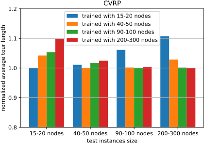
Next we evaluate the generalization performance of the agents to instances outside the training distribution. We tested each of the four CVRP agents, trained on the four instance size classes, on each of the four corresponding test sets. The results are depicted in Figure 1. For each test set, the agent trained on the respective training set performs best, and the agent trained on the smallest instances does not generalize well. For the other agents, the performance is not far away from the "specialists" for the respective instance sizes.
| ITR | GRD | 15-20 | 40-50 | 90-100 | 2-300 | |
|---|---|---|---|---|---|---|
| A | 43.0 | 43.9 | 42.1 | 41.9 | 41.6 | 42.1 |
| B | 42.3 | 42.4 | 41.1 | 41.1 | 39.8 | 40.1 |
| CMT | 74.8 | 65.2 | 70.7 | 68.6 | 62.7 | 63.6 |
| E | 33.6 | 31.4 | 32.2 | 30.9 | 30.0 | 30.4 |
| F | 45.0 | 47.5 | 40.9 | 40.6 | 43.0 | 41.3 |
| Gldn | 343.3 | 301.3 | 341.0 | 332.7 | 328.4 | 326.9 |
| M | 98.8 | 86.1 | 94.2 | 91.8 | 83.1 | 82.5 |
| P | 30.6 | 29.0 | 29.0 | 28.4 | 28.3 | 28.3 |
| X | 456.5 | 464.1 | 476.5 | 467.6 | 464.2 | 461.6 |
| RL | optimum | approx. factor | |
|---|---|---|---|
| CVRP | 12.26 | 11.30 | 1.09 |
| TSP | 5.32 | 5.19 | 1.03 |
We also evaluate the four trained CVRP agents on the CVRPlib data sets. Table 3 shows that for most of these standard benchmarks our RL agents exhibit good performance for the robust objective. The agent trained on instances with 90100 nodes appears to be the most universal choice.
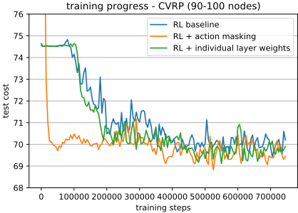
In a further experiment we look at two algorithm variants. In one variant we are masking infeasible actions using Equation 5. In the second variant each convolution layer is parameterized by individual weights. In Figure 2 the training progress in terms of the test cost is compared between the RL baseline and the two variants trained on the CVRP dataset with 90-100 nodes. While there is only little effect on the final performance, we find that action masking leads to substantially faster convergence time. This effect can also be observed on the other instance sizes. However, this effect does not generalize to TSP, as observed in another experiment 5 .
We finally compare the solutions computed by the RL agent (trained with instance size 90-100) to the solutions obtained from the mixed-integer problem formulation, where one hour of CPU runtime was admitted for the MIP solver. For each of the synthetic datasets, we have run the solver on 30 out of the 1,000 randomly generated instances, while we have included most datasets from CVRPlib and applied the solver to each instance from the selected datasets. The results are displayed in Table 5. On most datasets, the MIP based approach beats the RL approach. Recall however that the solver has one hour of computation time to search for a solution, while the trained RL agents return a solution within a single pass, which takes at most seconds.
6 Summary and Conclusion
We have presented an RL-based methodology to solve robust combinatorial optimization problems. Our agents are trained using feedback from exact evaluation of the robust objective.
5 The experiment will be provided in the long paper version.
| RL | MIP_1h | |
|---|---|---|
| VRP 15-20 nodes | 13.11 | 11.31 |
| VRP 40-50 nodes | 32.2 | 29.41 |
| VRP 90-100 nodes | 66.04 | 63.81 |
| VRP 200-300 nodes | 190.47 | 247.39 |
| CVRPlib-A | 41.63 | 39.29 |
| CVRPlib-B | 39.84 | 37.25 |
| CVRPlib-CMT | 62.66 | 69.27 |
| CVRPlib-E | 30.0 | 28.51 |
| CVRPlib-F | 42.97 | 45.47 |
| CVRPlib-Golden | 328.45 | 241.34 |
| CVRPlib-M | 83.09 | 96.74 |
| CVRPlib-P | 28.3 | 26.37 |
The agents learn to optimize a tight lower bound on the solution value in face of uncertainty, which is assisted by an environment which provides rewards based on the advantage over a baseline policy. Our experiments demonstrate that the trained agents are able to provide near-optimal solutions to min-max routing problems. Masking of infeasible actions can help to speed up training, and we observed that the agents generalize well to unseen distributions of problem instances.
We remark that the evaluation of both the baseline heuristic and the robust objective function in every training step represents a computational overhead as compared to non-robust optimization. An alternative approach to provide robustness guarantees could be to train a secondary agent to minimize lower bounds on ¯ f in the form of dual solutions.
Disclaimer The content of this work does not reflect the official opinion of the European Union. Responsibility for the information and views expressed therein lies entirely with the authors.
Acknowledgements
This project has received funding from the European Union's Horizon 2020 research and innovation programme under grant agreement No 769141.
@inproceedings{ijcai2021p357,
  title     = {Reinforcement Learning for Route Optimization with Robustness Guarantees},
  author    = {Jacobs, Tobias and Alesiani, Francesco and Ermis, Gulcin},
  booktitle = {Proceedings of the Thirtieth International Joint Conference on
               Artificial Intelligence, {IJCAI-21}},
  publisher = {International Joint Conferences on Artificial Intelligence Organization},
  editor    = {Zhi-Hua Zhou},
  pages     = {2592--2598},
  year      = {2021},
  month     = {8},
  note      = {Main Track},
  doi       = {10.24963/ijcai.2021/357},
  url       = {https://doi.org/10.24963/ijcai.2021/357},
}
TY - CPAPER TI - Reinforcement Learning for Route Optimization with Robustness Guarantees AU - Jacobs, Tobias AU - Alesiani, Francesco AU - Ermis, Gulcin T2 - Proceedings of the Thirtieth International Joint Conference on Artificial Intelligence, IJCAI-21 PB - International Joint Conferences on Artificial Intelligence Organization PY - 2021 SP - 2592 EP - 2598 DO - 10.24963/ijcai.2021/357 UR - https://doi.org/10.24963/ijcai.2021/357 ER -Copied
Machine-readable versions of this paper, for tools and AI agents:





