
State-Based Recurrent SPMNs for Decision-Theoretic Planning under Partial Observability
Proceedings of the Thirtieth International Joint Conference on Artificial Intelligence. Main Track. Pages 2526-2533.
https://doi.org/10.24963/ijcai.2021/348
Keywords
- Planning and Scheduling: Model-Based Reasoning
- Planning and Scheduling: Planning under Uncertainty
- Machine Learning: Learning Graphical Models
Abstract
The sum-product network (SPN) has been extended to model sequence data with the recurrent SPN (RSPN), and to decision-making problems with sum-product-max networks (SPMN). In this paper, we build on the concepts introduced by these extensions and present state-based recurrent SPMNs (S-RSPMNs) as a generalization of SPMNs to sequential decision-making problems where the state may not be perfectly observed. As with recurrent SPNs, S-RSPMNs utilize a repeatable template network to model sequences of arbitrary lengths. We present an algorithm for learning compact template structures by identifying unique belief states and the transitions between them through a state matching process that utilizes augmented data. In our knowledge, this is the first data-driven approach that learns graphical models for planning under partial observability, which can be solved efficiently. S-RSPMNs retain the linear solution complexity of SPMNs, and we demonstrate significant improvements in compactness of representation and the run time of structure learning and inference in sequential domains.
- [Bhattacharjya and Shachter, 2012] Debarun Bhattacharjya and Ross D Shachter. Evaluating influence diagrams with decision circuits. arXiv preprint arXiv:1206.5257, 2012.
- [Brockman et al., 2016] Greg Brockman, Vicki Cheung, Lud- wig Pettersson, Jonas Schneider, John Schulman, Jie Tang, and Wojciech Zaremba. OpenAI Gym. arXiv preprint arXiv:1606.01540, 2016.
- [Darwiche, 2003] Adnan Darwiche. A differential approach to inference in bayesian networks. Journal of the ACM (JACM), 50(3):280-305, 2003.
- [Ernst et al., 2005] Damien Ernst, Pierre Geurts, and Louis Wehenkel. Tree-based batch model reinforcement learning. Journal of Machine Learning Research, 6:503-556, 2005.
- [Fujimoto et al., 2019a] Scott Fujimoto, Edoardo Conti, Mo- hammad Ghavamzadeh, and Joelle Pineau. Benchmark- ing batch deep reinforcement learning algorithms. arXiv preprint arXiv:1910.01708, 2019.
- [Fujimoto et al., 2019b] Scott Fujimoto, David Meger, and Doina Precup. Off-policy deep reinforcement learning without exploration. In Proceedings of the 36th Interna- tional Conference on Machine Learning, pages 2052-2062, 2019.
- [Hoey et al., 1999] Jesse Hoey, Robert St-Aubin, Alan J Hu, and Craig Boutilier. Spudd: Stochastic planning using deci- sion diagrams. In Proceedings of Uncertainty in Artificial Intelligence, Stockholm, Sweden, 1999.
- [Howard and Matheson, 1984] Ronald A. Howard and James E. Matheson. Influence diagrams. In Ronald A. Howard and James E. Matheson, editors, The Principles and Applications of Decision Analysis. Strategic Decisions Group, Menlo Park, CA 94025, 1984.
- [Huang et al., 2006] Jinbo Huang, Mark Chavira, and Adnan Darwiche. Solving map exactly by searching on compiled arithmetic circuits. In AAAI, volume 6, pages 3-7, 2006.
- [Kaelbling et al., 1998] Leslie Pack Kaelbling, Michael L. Littman, and Anthony R. Cassandra. Planning and act- ing in partially observable stochastic domains. Artificial Intelligence, 101(1):99 -134, 1998.
- [Koller and Friedman, 2009] Daphne Koller and Nir Fried- man. Probabilistic graphical models: principles and tech- niques. MIT press, 2009.
- [Lange et al., 2012] Sascha Lange, Thomas Gabel, and Mar- tin Riedmiller. Batch reinforcement learning. In Marco Wiering and Martijn van Otterlo, editors, Reinforcement Learning: State-of-the-Art. Springer Berlin Heidelberg, 2012.
- [Lin, 1992] Long-Ji Lin. Self-improving reactive agents based on reinforcement learning, planning and teaching. Machine Learning, 8(293-321), 1992.
- [Melibari et al., 2016a] Mazen Melibari, Pascal Poupart, and Prashant Doshi. Sum-product-max networks for tractable decision making. In TWenty-Fifth International Joint Con- ference on Artificial Intelligence (IJCAI), pages 1846-1852, 2016. IJCAI
- [Melibari et al., 2016b] Mazen Melibari, Pascal Poupart, Prashant Doshi, and George Trimponias. Dynamic sum product networks for tractable inference on sequence data. In International Biennial Conference on Probabilistic Graphical Models (PGM), JMLR: Workshop & Conference Proceedings, Vol 52, pages 345-355, 2016.
- [Molina et al., 2019] Alejandro Molina, Antonio Vergari, Karl Stelzner, Robert Peharz, Pranav Subramani, Nicola Di Mauro, Pascal Poupart, and Kristian Kersting. Spflow: An easy and extensible library for deep probabilistic learning using sum-product networks. arXiv preprint arXiv:1901.03704, 2019.
- [Poon and Domingos, 2011] Hoifung Poon and Pedro Domingos. Sum-product networks: A new deep architec- ture. In 12th Conf. on Uncertainty in Artificial Intelligence (UAI), pages 2551-2558, 2011.
- [Sanner, 2010] Scott Sanner. Relational dynamic influence diagram language (rddl): Language description. 2010.
- [Tatavarti et al., 2021] Hari Teja Tatavarti, Prashant Doshi, and Layton Hayes. Data-driven decision-theoretic plan- ning using sum-product-max networks. In Proceedings of International Conference on Automated Planning and Scheduling (ICAPS), 2021.
References were extracted automatically from the PDF and may contain errors.
Full text extracted automatically from the PDF; figures, tables and equations may differ. The PDF is the version of record.
1 Introduction
Bayesian networks (BN) and their extensions, influence diagrams (ID) [Howard and Matheson, 1984], are frameworks for modeling probabilistic dependencies within multivariate distributions over various problem classes. These models are traditionally handcrafted and inference over even small networks is generally intractable. Arithmetic circuits (AC) [Huang et al., 2006], which can be compiled from BNs offer better certainty over the complexity of inference by using a computationoriented tree structure to model the inference problem. Most inference in ACs is linear in the size of the network, a significant improvement over the exponential inference complexity of BNs. Later, sum-product networks (SPN) [Poon and Domingos, 2011] were developed as a way to efficiently learn similar structures (linearly reducible to each other) directly from data.
Just as IDs generalize BNs, decision circuits (DC) [Bhattacharjya and Shachter, 2012] and their SPN-based analog, sum-product-max networks (SPMN) [Melibari et al., 2016a], extend the AC and SPN frameworks, respectively, to model probabilistic decision-making domains, allowing for inference and calculation of maximum expected utility over these domains in time linear in the size of the network. Melibari et al. [2016a] shows that SPMNs are efficiently reducible to DCs in time that is linear in the size of the SPMN. Likewise, recurrent SPNs (RSPN) [Melibari et al., 2016b] generalize SPNs in the same way that dynamic BNs extend BNs, providing a framework for learning graphical models for sequential domains. Most inference in RSPNs is linear in the size of the network, but by exploiting the recurrent structure of sequential domains through a repeated template network, RSPNs dramatically reduce the structure size required to model sequential data, thus improving inference speed. However, no dynamic extension of DCs to sequential contexts has been presented.
We present the (belief) state-based recurrent SPMN (SRSPMN) which exploits the recurrent structure in sequential decision-making (planning) problems. S-RSPMNs draw inspiration from the recurrent template that RSPNs add to SPNs to provide an analogous generalization of SPMNs, with a focus on partially-observed contexts. An S-RSPMN template can be viewed as a collection of interlinked SPMN structures, whose links can be followed to repeat the structure and model sequences of arbitrary lengths. We adapt the invariance property of RSPN's templates to ensure that an S-RSPMN is valid.
To guide the learning of the template's substructures and generate links between them, we utilize a data augmentation and state matching process, which serves to identify distinct belief states within the problem domain and their transitions. The substructures of an S-RSPMN are learned similarly to learning an SPMN. We test the performance of the learning algorithm by learning S-RSPMNs on a testbed of several sequential decision-making domains from OpenAI's Gym [Brockman et al., 2016] and RDDLSim [Sanner, 2010], demonstrating that they result in nearly optimal policy values for each. We also demonstrate competitive performance of policies learned by S-RSPMNs against a recent neural network approach, batchconstrained Q-learning [Fujimoto et al., 2019b], on the testbed. S-RSPMNs are thus a novel model-based representation for decision-theoretic planning in environments possibly partially observed, and which can be learned directly from offline data.
2 Background on SPMNs
SPNs [Poon and Domingos, 2011] are generative probabilistic graphical models, which can be learned directly from data.
Their simple structure, along with some validity constraints, means that probabilities for given evidence can be correctly computed in time linear in the size of the network for most types of queries (an exception are marginal MAP queries).
An SPN represents a joint probability distribution over its variables X1, X2, . . . , Xn. It is a rooted directed acyclic graph (DAG) whose leaves are the distributions of the random variables and whose internal nodes are sums and products. Each outgoing edge from a sum node has a non-negative weight. The value of a product node is the product of the values of its children while the sum node's value is the weighted sum of its children's values. The value of a SPN is the value of its root which can be represented as a network polynomial [Darwiche, 2003]. The SPN is valid iff the normalized polynomial represents the joint distribution of the variables and produces the correct marginals. The scope of a node is the union of scopes of its children. A leaf node's scope is the set of random variables whose distribution it holds.
The validity of an SPN is sufficiently ensured if it adheres to the following constraints on the scopes of various nodes.
Definition 1 (Sum-complete). An SPN is sum-complete iff each children of the same sum node have an identical scope.
Definition 2 (Decomposable). An SPN is decomposable iff no variable appears in more than one child of a product node.
These properties permit the following theorem.
Theorem 1 (SPN validity [Poon and Domingos, 2011]). An SPN is valid if it is sum-complete and decomposable.
However, Melibari et al. [2016b] show that these models scale poorly when applied to sequential domains. As the number of variables increases with the number of steps in the sequence, the learned SPN exhibits an exponential increase in structure size, learning time, and inference time.
SPMNs [Melibari et al., 2016a] extend SPNs by adding max and utility nodes, analogously to the extension of BNs to IDs. By adding these node types, along with some additional validity constraints, SPMNs enable modeling of probabilistic decision-making problems and computing the policy in time linear in the size of the network.
Definition 3 (SPMN). An SPMN over random variables X1, . . . ,Xn, decision variables D1, . . . ,Dm, and utility functions U1, . . . ,Uk is a rooted DAG. Its leaves are either distributions of the random variables or utility nodes that hold constant values. An internal node of an SPMN is either a sum, product, or max node. Each max node corresponds to one of the decision variables and each outgoing edge from a max node is labeled with one of the possible values of the corresponding decision variable. Value of a max node i is maxjϵChildren(i)vj, where Children(i) is the set of children of i, and vj is the value of the subgraph rooted at child j. The sum and product nodes are defined as in the SPN.
A valid SPMN is one whose evaluation results in the same maximum expected utility (MEU) as that obtained via application of the Sum-Max-Sum rule [Koller and Friedman, 2009]. This is ensured by the addition of the following sufficiency constraints [Melibari et al., 2016a].
Definition 4 (Max-completeness). An SPMN is max-complete iff all children of the same max node have the same scope, where the scope is as defined previously.
Definition 5 (Max-uniqueness). An SPMN is max-unique iff each max node that corresponds to a decision variable D appears at most once in every path from root to leaves.
Theorem 2 (SPMN validity [Melibari et al., 2016a]). An SPMN is valid if it is sum-complete, decomposable, maxcomplete, and max-unique.
An important concept related to SPMNs is that of the partial order of the variables. A partial order, denoted by P ≺, is an ordered list of information sets and decision variables. Information sets are subsets of the random variables of the problem domain. Partial orders take the form I0 ≺ D1 ≺ I1 ≺ D2 ≺ . . . ≺ Dm ≺ Im, where the variables of an information set Ii-1 are observed before decision variable Di, and the variables of Ii are observed only after the decision at Di is made. This is a partial ordering over the variables because the ordering of the variables in any information set is unspecified.
The partial order is respected while learning the structure of an SPMN in that the variables of information set Ii-1 are outside the scope of the decision node corresponding to decision variable Di (coming earlier in the structure), whereas all variables Ii, Ii+1, . . ., are within its scope.
MEU calculation in an SPMN is performed by propagating the values of each utility node along side the probabilities. First, the leaf nodes consistent with the given evidence are set to 1 and the rest to zero. Then the structure is evaluated bottom-up, where the operators at each node are applied to the values of the children. In this way, the expected value at each node is determined, with the overall MEU collected at the root. To determine the optimal decision values given the evidence, the network can then be traversed top-down, selecting the decisions corresponding to the child with greatest expected utility at each decision node.
This complexity of the evaluation is thus linear with the number of nodes in the network. However as with SPNs, the number of nodes in the structure may grow exponentially with the number of variables, rendering SPMNs largely intractable in many sequential decision-making domains.
3 State-Based Recurrent SPMNs
A straightforward generalization of RSPNs to decision-making problems thereby yielding recurrent SPMNs exists [Tatavarti et al., 2021], but this targets contexts whose state is perfectly observed. In contrast, we aim to introduce a model for partially-observable environments where the data consists of noisy observations (not values of state variables), which complicates the generalization.
The planning data for learning S-RSPMNs consists of a finite temporal sequence of values of observation, decision, and utility variables. Formally, consider a partiallyobserved decision-making problem where the state of the environment is informed by n observation variables, Ω1, Ω2, . . ., Ωn; decisions by a combination of m decision variables, D1, D2, . . ., Dm; and a single utility variable U. A candidate data record of at most T steps is then a sequence of T tuples of the form 〈(I0, d1, I1, d2, . . . , Im-1, dm, Im, u)0 , (I0, d1, I1, d2, . . . , Im-1, dm, Im, u)1 , . . ., (I0, d1, I1, d2, . . . , Im-1, dm, Im, u)T-1 )〉. Here, I0, I1, . . . , Im are information sets, as mentioned in Section 2, but where Ii-1, 1 ≤ i ≤ m consists of values of the observation variables in the information set of Di. Additionally, u in each tuple is the value of utility variable U given the realizations of the hidden state variables and observed decisions in that tuple. Next, we define the template, a key component of S-RSPMNs.
Definition 6 (S-RSPMN template). A template network for a slice of n observation variables at time t is a DAG with k roots and k + l + n leaf nodes, where k > 0, l > 0. The n leaf nodes hold the distributions over observation variables, Ωt1 , Ωt2 , . . . , Ωtn or hold constant values as utility nodes. The remaining k and l leaves consist of two types of distinguished nodes, respectively denoted as S1 and S2. Each of the k roots is a product node which has exactly one S1 node as a direct child and contains at least one S2 node in its scope. The interior nodes of the template consist of sum, product, and max nodes and the edges have their usual semantics.
The template network can be viewed as a collection of interlinked SPMN substructures, each of which we refer to as a state estimation branch. Each such branch is rooted at a product node and corresponds to a distinct belief region in the problem with its S1 node containing a collection of integer labels. Each S2 leaf node in the template links to the state branch whose S1 node contains its label. These links represent the transition from one belief region to another at the conclusion of a step of the sequence.
Next, we introduce the top and bottom networks, which allow the S-RSPMN to yield a rooted SPMN when the templates are repeated as many times as the length of the sequence data.
Definition 7 (Top network). A top network is a rooted DAG whose root is a sum node with k leaves as children. Leaves of this network are interface nodes, each of which will be merged with a distinct root of the template. Each edge (i, j) emanating from the root sum node has a non-negative weight wij. A bijective mapping g determines which root of the template corresponds to an interface node of the top network.
Definition 8 (Bottom network). A bottom network modeling the last time slice of n observation variables, 〈Ω1, Ω2, . . . , Ωn〉T , is similar to the template network with k roots but k + n leaf nodes. No S2 nodes are present.
To model sequential decision-making data of length T , we construct an S-RSPMN by learning the top and template networks. Then, T - 1 instances of the template network are stacked on the bottom network, and capped with a top network. To stack instances of the template network, each S2 node is replaced with the root node of the template's state estimation branch whose S1 node contains its value. The top network is then merged with this structure by replacing its interface nodes with the corresponding roots as mapped by g.
The validity of an S-RSPMN over any number of steps can be established by repeating the template, as described above, to the desired number of steps and verifying the conditions given in Defs. 1, 2, 4, and 5 for each node. However, we may define a property to allow establishing the validity without unrolling the network. This property is inspired by the template invariance property of RSPNs [Melibari et al., 2016b].
Definition 9 (Template soundness). The template network presented in Def. 6 is sound iff (a) the scope of the structure replacing each S2 node excludes St1 , Ωt1 , ..., Ωtn , and is identical to the scope of each other such structure, (b) all product nodes in the template network are decomposable, (c) all sum nodes in the template are complete, and (d) all max nodes in the template are both max-complete and max-unique.
This property is helpful in proving the validity of a network in that the roots of a sound template satisfy the conditions of soundness when they are used to replace the S2 nodes of another copy of the same template network modeling the previous step of the sequence. Theorem 3 shows that this property can be used to establish the validity of an S-RSPMN modeling an arbitrary number of steps.
Theorem3 (S-RSPMNvalidity). If the (a) top network is sumcomplete and bottom network is sum- and max-complete, maxunique, and decomposable, (b) scope of each state branch in the bottom network is identical to the scope of every other such branch, and (c) S2 nodes can be replaced with corresponding state branches in such a way that the template network is sound, then the corresponding S-RSPMN is valid.
The proof, given in the technical appendix included in the supplement, is established by induction on the sequence length and observing that the conditions (a-c) always yield an unrolled SPMN that is valid.
4 Learning S-RSPMN fromData
Sequential decision-making problems can be modeled using SPMNs without recurrence by simply blocking the entire sequence of tuples in a record as one data input and applying the LearnSPMN algorithm of Melibari et al [2016b]. However, as our experiments demonstrate, this approach often results in very large structures whose size is exponential in the number of variables, and also exponential in the number of time steps of a sequence. This proves intractable for longer sequences. Furthermore, the SPMNs once learned are unable to model any newer sequences whose length is greater than the longest sequences in the training data.
Consequently, there is strong motivation for an algorithm that automatically learns the structure of an S-RSPMN template and top networks, such that the structure satisfies the property of soundness given in Def. 9. Overall, our method for learning the S-RSPMN structure iteratively applies LearnSPMN over small numbers of steps to learn multiple SPMN substructures. These are linked together through a matching process to form a recursive structure.
To help illustrate the process, we introduce a simple sequential decision-making problem, the repeated marbles game. It starts with a bag containing 2 marbles, one white and the other black, unknown to the agent. The agent can chose to either draw a marble randomly or to reset the problem to the initial state. The problem is also automatically reset to the initial state once both marbles are drawn. Drawing the white marble results in +1 utility, whereas drawing the black marble results in -1 utility, so the optimal play is to draw until the white marble is found and then reset the problem, resulting in an average of +0.5 utility per 2 steps of the problem. The state is represented by a single variable, X, that corresponds to which marble is left in the bag. The drawn marble is observed perfectly thereby yielding a single observation variable Ω. A single decision variable draw involves choosing one of two actions: draw a marble or reset.
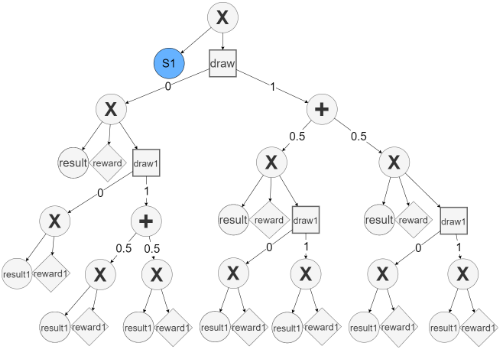
Algorithm 1 gives the main procedure, LEARNS-RSPMN, for learning the S-RSPMN template. As we may expect, LEARNS-RSPMN takes the set D of records each containing a sequence of tuples and a partial order over the domain variables P ≺. Additionally, two learning parameters need to be pre-specified: (i) the horizon, h, which is the number of time steps considered in each application of the underlying LearnSPMN. Increasing h allows us to model longer-term dependencies but doing so will also increase the run time of the algorithm. (ii) The correlation threshold cthresh is used in the matching process to determine whether a correlation between an existing substructure and variable values is not sufficiently significant thereby necessitating a new substructure.
The algorithm begins by augmenting each data record (lines 1-4). It prepends an additional variable to the partial order of each step of a sequence, labeled as S1. The variable takes a state identifier (SID) as its value. Specifically, each augmented tuple in the data record takes the form (S1, I0, d1, I1, d2, . . . , Im-1, dm, Im, u)t . SID for the S1 in the initial time-step tuple of each record is 0, signifying the initial region. The S1 values for each subsequent step is set based on an evaluation of the network over its preceding step in a process described later.
Next, we learn the first substructure by applying LearnSPMN to the tuples of the first h time steps of each data record (line 5). This learns a state estimation branch for the initial state of the sequence, SID 0. As S1 is first in the partial order and takes only one value in the data, it is always a child of a root product node. We illustate the state estimation branch with SID 0 for the repeated marbles game in Fig. 1.
Algorithm 1: LEARNS-RSPMN
Input: Data set: D = 〈τ 0 , τ 1 , . . . , τ T-1 〉e where e = 1, 2, . . . , E
Partial order over all variables for two steps: P ≺, Horizon: h ▷ number of steps used in structure learning and branch matching Correlation threshold: cthresh
Output: learned S-RSPMN
- 1 Prepend a column for SID, Se,t 1 , to each tuple τ t in each episode e of D with NULL value
- 2 Prepend a new information set containing only SID to each time step of P ≺
- 3 Set SID for the initial tuple τ 0 e of each episode e, Se,0 1 ← 0
- 4 numSIDs ←1, SIDtoBranch←newmap
- 5 SPMN0 ←LEARNSPMN(D0:h-1 , P ≺)
- 6 SPMN0 , numSIDs ←REPLACEBRANCHES(SPMN0 , P ≺, numSIDs)
- 7 SIDtoBranch[0] ←SPMN0
- 8 S-RSPMN← new root sum node with SPMN0 as its child ▷ top network
9 do
10 D, maxDataSID←UPDATEDATACOUNTS(D,
SIDtoBranch, numSIDs)
11 matched←False
12
13
14
15
16
17
18
19
20
21
22
23
24
for branch in the children of S-RSPMN do
if BRANCHMATCH(D, branch, maxDataSID, h,
cthresh) then
add maxDataSID to the list of SIDs in the S1 node of branch
SIDtoBranch[maxDataSID] ← branch matched ← True
exit for loop
if not matched then
newBranchData ← 〈τ t , . . . , τ t+h-1 〉e for each tuple τ t and episode e in D where Se,t 1 = maxTuplesSID SPMNs ← LEARNSPMN(newBranchData, P ≺) SPMNs , numSIDs ← REPLACEBRANCHES(SPMNs , P ≺, numSIDs)
S-RSPMN← add SPMNs as a new child of the root sum node of S-RSPMN
update weights of the root sum node of S-RSPMN SIDtoBranch[maxDataSID] ← newBranch
- 25 while maxDataSID is not NULL
- 26 return S-RSPMN
While this SPMN models data over multiple time steps, recall that the template focuses on one time step only. We include the additional h - 1 steps in the learning (rather than focusing on the data at time step 0 only) to model the subsequent transitions, which ensures sufficient branching in the structure as we see in Fig. 1. Taking a step toward creating the template, the additional structure is then pruned away and replaced by S2 nodes (line 6). These nodes replace the first occurrence of a variable from the next time step (often the decision variable as in the example). Each new S2 is assigned a value that is incremented by 1, starting at 1. Algorithm 2 REPLACEBRANCHES included in the supplement gives the procedure of replacing the branches rooted at such variables with S2 nodes. This creates a simpler structure, as we illustrate
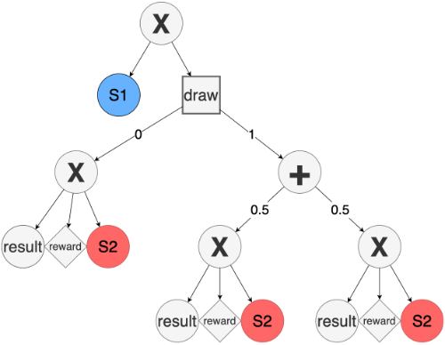
in Fig. 2 for the marbles game.
This first substructure is added as a child to a new sum node which serves as the root of the template network. The resulting structure is sufficient to model only the first state of the problem. In order to model additional states and the transitions between them, we use the newly created S2 nodes to augment the next step tuple of data with SID values. Each S2 node represents a state transition, and its corresponding SID value will serve to tell us to which state estimation branch it connects.
For each sequence, we determine the SID value of its next step by finding the S2 node reached by the current step. Toward this, we obtain the S2 node that yields the maximum likelihood for the state estimation branch for the current timestep tuple. We obtain this by assigning a value of 1 to each S2 node in turn and assigning other S2 nodes a value of 0. Then, calculate the likelihood for the data in the current tuple, say time step 0, and select the S2 node that was assigned 1, which yielded the largest likelihood. This is analogous to selecting the S2 node yielding the most probable explanation (line 8 of Algorithm 3 UPDATEDATACOUNTS included in the supplement). This S2 node's value is then assigned as the SID value of S1 in the next time-step tuple in that record. We do this for each record in the data set.
On assigning the SID for the next step of each record, LEARNS-RSPMN attempts to match the next-step data tuples containing the new SID values to existing state estimation branches in lines 12-13 of the algorithm. This is done by combining data tagged with the new SID value with the data tagged by SID values contained in a branch, then detecting correlations within that combined data (Algorithm 4 BRANCHMATCH in the supplement). If SID in this combined dataset is correlated with any other variable (excluding decisions), then we move on to the next branch. If for a given branch, the SID is not correlated with the other variables, then the belief state represented by this SID is indistinguishable from the state modeled by that branch, making it a match.
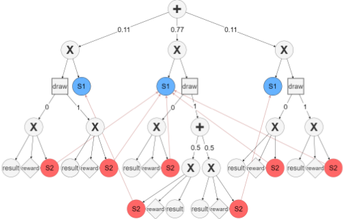
Figure 3: Final S-RSPMN structure learned for the repeated marbles game. Red dotted line between S1, S2 node pair indicates that the S1 node contains the value of the linked S2 SID. The S-RSPMN consists of the template network with three state estimation branches, whose roots are the product nodes in the second layer from the top. The top network connects the root sum node with the three product nodes. Weights on the edges correspond to the relative frequency with which belief states in each region are encountered in the data.
If a match is found, we add the SID value to the set of SIDs held by the S1 node of the matching branch (lines 14-15 of Algorithm 1). This indicates that the belief region represented by the matched state estimation branch covers the belief represented by the data sequence. If no match is found (lines 18-24), then the SIDmay represent a new belief state. In that case, we learn a new SPMN substructure. First, the learning data is comprised of the tuple at time step t that did not match, tuples at step t from other records whose S1 value is identical to the SID, and the tuples of the next h - 1 steps in each data record (or until the last time step if it is reached prior to h). We apply LearnSPMN to this data subset to obtain a new state estimation branch. As before, we replace the subgraphs whose scopes fall outside the set of variables at time step t with new S2 nodes. The resulting SPMN substructure is added as a new child of the root sum node of the template network. Weights on the edges are equal and correspond to a uniform distribution.
The matching process is performed for the next tuple in each data record. If a new SPMN substructure is learned, S2 nodes corresponding to the most probable explanation are found and the matching process is repeated as we move across all the time steps of the data. Figure 3 shows a complete, fully-linked S-RSPMN for the repeated marbles game with three stateestimation branches each corresponding to a distinct belief region - for the states where both marbles are in the bag and the black or white marble only remains in the bag.
SIDs of most likely S2 nodes based on the last time-step tuple cannot be assigned forward to the next S1 node as there is no further tuple of data. Nevertheless, we must assign them to some S1 node(s) to model the transition in the belief state. Our approach is to add the S2 node's value to the set of SIDs held in the S1 nodes of all the state-estimation branches in the template. This is analogous to modeling the transition to a distribution of next belief regions.
| Data set | |X|, |Ω|, |D| | #Episodes | T | #Columns |
|---|---|---|---|---|
| Repeated marbles | (1, 1, 1) | 5K | 6 | 18 |
| Tiger problem | (1, 1, 1) | 100K | 7 | 21 |
| NChaina | (1, 1, 1) | 100K | 10 | 30 |
| Frozen lakea | (1, 1, 1) | 100K | 10 | 30 |
| Skill teachingb | (12, 4, 4) | 500K | 10 | 90 |
| Elevatorsb | (13, 5, 4) | 500K | 10 | 100 |
| Crossing trafficb | (18, 3, 4) | 500K | 10 | 80 |
| Navigationb | (15, 4, 4) | 500K | 10 | 90 |
5 MEU Evaluation
A brute force approach to MEU evaluation in an S-RSPMN would be to unroll the structure to the desired planning horizon by recursively replacing the S2 nodes with their matching branch - this is the branch whose S1 node contains the S2 node's SID value. However, we can dramatically speed up the MEU evaluation by exploiting the recurrent properties of the network with dynamic programming. Beginning at the last time step (horizon 1), we prune the template to yield the bottom network (Def. 8). The MEU for each state-estimation branch is then the highest EU at the product nodes that form the roots of the branches in the bottom network, using a bottom-up pass through each branch. We may associate these MEUs with the identifying S1 nodes of the branches.
To calculate the value of a state-estimation branch for two steps of unconditioned evaluation, we iterate through each possible decision path in the branch and add the weighted sum over the S2 nodes reachable in that path to the single step value of the path. The value of an S2 node here is equal to the single-step value of the state-estimation branch to which it is linked. This value was computed as mentioned in the previous paragraph. For each branch, we then take the largest combined value from among its possible decision paths as the MEU value for that branch for a horizon of two. This procedure is repeated, using the branch values for two steps to obtain the values for a horizon of three, and so on, to the specified T . By memoizing the MEU values for each branch and time step, we can quickly determine the unconditioned MEU up to any T. This effectively reduces the run time complexity from O(bT ) to O(lbm) where b is the worst-case branching factor of the network, and the remaining parameters are as defined in Section 2.
6 Experiments
The LEARNS-RSPMN algorithm has been implemented in the SPFlow library [Molina et al., 2019] and is available on GitHub at https://github.com/minimum-LaytonC/SPFlow/tree/
| S-RSPMN | SPMN | |||||
|---|---|---|---|---|---|---|
| Domain | T | #Episodes | Learn time | #nodes | Learn time | #nodes |
| Repeated | 3 | .1K | 1.77s | 39 | 2.61s | 85 |
| marble | 4 | 1K | 2.44s | 39 | 6.19s | 274 |
| 5 | 1K | 2.53s | 39 | 17.24s | 615 | |
| 6 | 5K | 6.67s | 39 | 56.94s | 1,710 | |
| Tiger | 3 | 10K | 25s | 147 | 22s | 250 |
| 4 | 100K | 147s | 229 | 174s | 1,673 | |
| 5 | 100K | 212s | 213 | 684s | 8,027 | |
| 6 | 100K | 240s | 237 | 2153s* | 28,408 | |
| 7 | 100K | 230s | 221 | 5402s* | 75,046 | |
rspmn rdc rmeufix under the Apache license. We evaluate its performance on a new testbed of sequential decision-making data sets that adhere to the schema given in Section 3 and where the state is partially observed.
As there are very few existing data sets on simulations of discrete partially observable decision-making domains, we developed a new testbed of eight data sets on decision-making problems, listed in Table 1 and available at https://github.com/ minimum-LaytonC/SRSPMN dataset generators. In addition to the repeated marbles game, we also include simulations of the Tiger problem, a well-known POMDP domain [Kaelbling et al., 1998]. Two of the remaining data sets are simulations of the NChain and Frozen lake domains, which are fully-observable problems (where observation variables are synonymous with state variables) sourced from OpenAI's Gym [Brockman et al., 2016]. The remaining four data sets (Crossing traffic, Elevators, Skill teaching, and Navigation) are simulations of larger RDDLSim POMDP domains [Sanner, 2010], which are partially observable. Each data set is generated by using a random policy which interacts with the environment and collecting the 〈action, observation, reward〉 generated at each step. Each episode is run until either the goal state or some other terminal state is reached, after which some of the domains automatically restart. Each episode generates a data record.
The advantages of S-RSPMNs over SPMNs in sequential domains can be seen clearly in their comparative performance on the toy repeated marbles and Tiger problems. Table 2 shows the learning times and structure sizes over several different sequence lengths T and numbers of episodes. We selected the number of episodes for each sequence length that is sufficient for both models to obtain MEU values that are optimal with some exceptions. The size of the S-RSPMN does not significantly change with increase in sequence length as the template structure learned is sufficient to model any number of steps. Observe that its learning time is effectively linear in the size of the data set. Contrast this with the exponential increase in learning time and structure sizes of the SPMNs with sequence lengths. While we may not see this level of improvement for other problems (many problems will have a larger space of belief regions that yield distinct behaviors), these simple problems serve to demonstrate the advantages of a recurrent model in terms of both time and compactness of representation. Indeed, we were unable to generate SPMNs for even small time steps for some of the other relatively larger domains with structure learning taking many hours before ultimately failing due to excessive memory requirements.
| S-RSPMN | BCQ | |||||||
|---|---|---|---|---|---|---|---|---|
| Domain | Optimal EU | MEU | Mean total reward | Learn time(s) | #nodes | 〈h, cthresh〉 | Mean total reward | Learn time(s) |
| NChain | 25.8 | 25.86 | 24.54 ± 0.26 | 111 | 106 | 〈2, 0.3〉 | 15.228 ± 0 | 32,196 |
| Frozen lake | 0.823 | 0.816 | 0.742 ± 0 | 4,081 | 649 | 〈3, 0.3〉 | 0.0 ± 0 | 37,878 |
| Skill teaching | 5.953 | -6.136 | 5.198 ± 0.98 | 17,020 | 1,447 | 〈3, 0.26〉 | -6.329 ± 0 | 34,247 |
| Elevators | -14.44 | -1.953 | -19.103 ± 0.22 | 4,941 | 1,324 | 〈3, 0.24〉 | -18.953 ± 0.85 | 36,620 |
| Crossing traffic | -3.909 | -3.28 | -5.635 ± 0.29 | 2,489 | 203 | 〈4, 0.22〉 | -19.882 ± 0 | 38,548 |
| Navigation | -7.713 | -5.809 | -8.025 ± 0 | 7,519 | 563 | 〈3, 0.30〉 | -8.025 ± 0 | 36,059 |
S-RSPMNs are related in principle to batch (or off-policy) reinforcement learning methods [Lin, 1992; Ernst et al., 2005; Lange et al., 2012]. Both these types of methods seek to derive an optimal policy from a given set of prior experiences though S-RSPMNs learn a model while the latter tend to be model free. Therefore, as a baseline, we compare with a recent offpolicy reinforcement learning technique constrained to learn from a batch of data, a discrete implementation of the batchconstrained deep Q-Learning (BCQ) [Fujimoto et al., 2019a; Fujimoto et al., 2019b] applied to the testbed. Table 3 reports on the performances of the learned S-RSPMN and BCQ for the Gym and RDDLSim data sets. The optimal EU for the Gym domains is provided by converged deep Q-networks while the symbolic Perseus solver [Hoey et al., 1999] provides the same for the RDDLSim domains. Clearly, a key question to ask is: how good are the policies learned by S-RSPMN and BCQ? We simulated the policies obtained from the learned models and report the mean ± standard deviation of the total reward across 10 runs of 100 episodes each. Table 3 shows that the mean rewards from S-RSPMNs are close to the optimal EU for all the domains, and the difference between the two is significantly less than or similar to that of the mean rewards from BCQ (the sole exception is Elevators). Simultaneously, learning times for S-RSPMNs are often an order of magnitude less than those of BCQ.
However, the learned S-RSPMNs yielded MEUs that did not always align with the rewards from policy simulation! This is evident for the partially-observed RDDLSim domains and indicates that an accurate model of the environment was not learned in these cases, possibly due to the absence of the state variables from the data. But, the MEUs were indeed computed quickly taking just 0.005s and 0.007s for the NChain and Frozen lake models, respectively.
7 Conclusion
Decision-theoretic planning has relied on accurately specifying the model and (optimal) planning remains intractable for all but the simplest problems. This paper seeks to address both these challenges by infusing data-driven machine learning into planning with a fundamental focus on tractability. Whereas the default approach for bringing efficiency to planning is approximations that trade off quality, our approach learns fitted problem representations that are guaranteed to solve efficiently. Task simulation data, which is seldom directly used for automated planning, can now be collected and used. A concomitant risk to this potentially high payoff is that the size of S-RSPMNs is unbounded. Furthermore, S-RSPMNs offer clear semantics for decision making in contrast to neural nets. A direction of future work is to develop anytime techniques for learning the networks, which offer flexible control over the size of the network while yielding structures with improving likelihoods and MEUs.
Acknowledgements
This research was supported by NSF grant #IIS-1815598. We thank Scott Sanner, Alan Fern, and Murugeswari Issakkimuthu for guidance in making our RDDLSim installation operational and for providing their Python RL interface to RDDL. We acknowledge the anonymous reviewers for their feedback.
@inproceedings{ijcai2021p348,
  title     = {State-Based Recurrent SPMNs for Decision-Theoretic Planning under Partial Observability},
  author    = {Hayes, Layton and Doshi, Prashant and Pawar, Swaraj and Tatavarti, Hari Teja},
  booktitle = {Proceedings of the Thirtieth International Joint Conference on
               Artificial Intelligence, {IJCAI-21}},
  publisher = {International Joint Conferences on Artificial Intelligence Organization},
  editor    = {Zhi-Hua Zhou},
  pages     = {2526--2533},
  year      = {2021},
  month     = {8},
  note      = {Main Track},
  doi       = {10.24963/ijcai.2021/348},
  url       = {https://doi.org/10.24963/ijcai.2021/348},
}
TY - CPAPER TI - State-Based Recurrent SPMNs for Decision-Theoretic Planning under Partial Observability AU - Hayes, Layton AU - Doshi, Prashant AU - Pawar, Swaraj AU - Tatavarti, Hari Teja T2 - Proceedings of the Thirtieth International Joint Conference on Artificial Intelligence, IJCAI-21 PB - International Joint Conferences on Artificial Intelligence Organization PY - 2021 SP - 2526 EP - 2533 DO - 10.24963/ijcai.2021/348 UR - https://doi.org/10.24963/ijcai.2021/348 ER -Copied
Machine-readable versions of this paper, for tools and AI agents:





