
Fine-Grained Air Quality Inference via Multi-Channel Attention Model
Proceedings of the Thirtieth International Joint Conference on Artificial Intelligence. Main Track. Pages 2512-2518.
https://doi.org/10.24963/ijcai.2021/346
Keywords
- Machine Learning: Time-series; Data Streams
Abstract
In this paper, we study the problem of fine-grained air quality inference that predicts the air quality level of any location from air quality readings of nearby monitoring stations. We point out the importance of explicitly modeling both static and dynamic spatial correlations, and consequently propose a novel multi-channel attention model (MCAM) that models static and dynamic spatial correlations as separate channels. The static channel combines the beauty of attention mechanisms and graph-based spatial modeling via an adapted bilateral filtering technique, which considers not only locations' Euclidean distances but also their similarity of geo-context features. The dynamic channel learns stations' time-dependent spatial influence on a target location at each time step via long short-term memory (LSTM) networks and attention mechanisms. In addition, we introduce two novel ideas, atmospheric dispersion theories and the hysteretic nature of air pollutant dispersion, to better model the dynamic spatial correlation. We also devise a multi-channel graph convolutional fusion network to effectively fuse the graph outputs, along with other features, from both channels. Our extensive experiments on real-world benchmark datasets demonstrate that MCAM significantly outperforms the state-of-the-art solutions.
- [Arystanbekova, 2004] N. Kh. Arystanbekova. Application of gaussian plume models for air pollution simulation at instantaneous emissions. Mathematics and Computers in Simulation, 67(4):451-458, 2004.
- [Chen et al., 2016] Ling Chen, Yaya Cai, Yifang Ding, Mingqi Lv, Cuili Yuan, and Gencai Chen. Spatially fine- grained urban air quality estimation using ensemble semi- supervised learning and pruning. In Proceedings of the 2016 ACM International Joint Conference on Pervasive and Ubiquitous Computing (UbiComp), pages 1076-1087, 2016.
- [Cheng et al., 2018] Weiyu Cheng, Yanyan Shen, Yanmin Zhu, and Linpeng Huang. A neural attention model for urban air quality inference: Learning the weights of mon- itoring stations. In Proceedings of the 32th AAAI Confer- ence on Artificial Intelligence (AAAI), pages 2151-2158, 2018.
- [Guizilini and Ramos, 2015] Vitor Guizilini and Fabio Ramos. A nonparametric online model for air quality prediction. In Proceedings of the 29th AAAI Conference on Artificial Intelligence (AAAI), pages 651-657, 2015.
- [Hochreiter and Schmidhuber, 1997] Sepp Hochreiter and Jürgen Schmidhuber. Long short-term memory. Neural Computation, 9(8):1735-1780, 1997.
- [Hsieh et al., 2015] Hsun-Ping Hsieh, Shou-De Lin, and Yu Zheng. Inferring air quality for station location recom- mendation based on urban big data. In Proceedings of the 21th ACM SIGKDD International Conference on Knowl- edge Discovery and Data Mining (KDD), pages 437-446, 2015.
- [Jutzeler et al., 2014] Arnaud Jutzeler, Jason Jingshi Li, and Boi Faltings. A region-based model for estimating urban air pollution. In Proceedings of the 28th AAAI Conference on Artificial Intelligence (AAAI), pages 424-430, 2014.
- [Li et al., 2017] Xiang Li, Ling Peng, Xiaojing Yao, Shao- long Cui, Yuan Hu, Chengzeng You, and Tianhe Chi. Long short-term memory neural network for air pollutant con- centration predictions: Method development and evalua- tion. Environmental Pollution, 231:997-1004, 2017.
- [Liang et al., 2018] Yuxuan Liang, Songyu Ke, Junbo Zhang, Xiuwen Yi, and Yu Zheng. Geoman: Multi-level attention networks for geo-sensory time series prediction. In Proceedings of the 27th International Joint Conference on Artificial Intelligence (IJCAI), pages 3428-3434, 2018. IJCAI
- [Luo et al., 2019] Zhipeng Luo, Jianqiang Huang, Ke Hu, Xue Li, and Peng Zhang. Accuair: Winning solution to air quality prediction for kdd cup 2018. In Proceed- ings of the 25th ACM SIGKDD International Conference on Knowledge Discovery and Data Mining (KDD), pages 1842-1850, 2019.
- [Rakowska et al., 2014] Agata Rakowska, Ka Chun Wong, Thomas Townsend, Ka Lok Chan, Dane Westerdahl, Si- mon Ng, Griša Močnik, Luka Drinovec, and Zhi Ning. Impact of traffic volume and composition on the air qual- ity and pedestrian exposure in urban street canyon. Atmo- spheric Environment, 98:260-270, 2014.
- [Tomasi and Manduchi, 1998] Carlo Tomasi and Roberto Manduchi. Bilateral filtering for gray and color images. In Proceedings of the 6th International Conference on Com- puter Vision (ICCV), pages 839-846, 1998.
- [Wilson et al., 2018] Tyler Wilson, Pang-Ning Tan, and Lifeng Luo. A low rank weighted graph convolutional ap- proach to weather prediction. In Proceedings of the 18th IEEE International Conference on Data Mining (ICDM), pages 627-636, 2018.
- [Yi et al., 2018] Xiuwen Yi, Junbo Zhang, Zhaoyuan Wang, Tianrui Li, and Yu Zheng. Deep distributed fusion network for air quality prediction. In Proceedings of the 24th ACM SIGKDD International Conference on Knowledge Discov- ery and Data Mining (KDD), pages 965-973, 2018.
- [Zhang et al., 2019] Yawen Zhang, Qin Lv, Duanfeng Gao, Si Shen, Robert P. Dick, Michael Hannigan, and Qi Liu. Multi-group encoder-decoder networks to fuse heteroge- neous data for next-day air quality prediction. In Proceed- ings of the 28th International Joint Conference on Artifi- cial Intelligence (IJCAI), pages 4341-4347, 2019. IJCAI
- [Zhao et al., 2017] Xiangyu Zhao, Tong Xu, Yanjie Fu, En- hong Chen, and Hao Guo. Incorporating spatio-temporal smoothness for air quality inference. In Proceedings of the 17th IEEE International Conference on Data Mining (ICDM), pages 1177-1182, 2017.
- [Zheng et al., 2013] Yu Zheng, Furui Liu, and Hsun-Ping Hsieh. U-air: When urban air quality inference meets big data. In Proceedings of the 19th ACM SIGKDD Interna- tional Conference on Knowledge Discovery and Data Min- ing (KDD), pages 1436-1444, 2013.
- [Zheng et al., 2015] Yu Zheng, Xiuwen Yi, Ming Li, Ruiyuan Li, Shan, Eric Chang, and Tianrui Li. Forecast- ing fine-grained air quality based on big data. In Proceed- ings of the 21th ACM SIGKDD International Conference on Knowledge Discovery and Data Mining (KDD), pages 2267-2276, 2015.
References were extracted automatically from the PDF and may contain errors.
Full text extracted automatically from the PDF; figures, tables and equations may differ. The PDF is the version of record.
1 Introduction
With the fast pace of industrialization and urbanization, air pollution has become a major public concern. To reduce the harmful effects of air pollution, accurately predicting air quality is of great importance for both governments and the public. The capability of providing fine-grained air quality inference is especially critical to, for example, guide people to make proper plans to avoid adverse effects on health through the air they breathe [Zheng et al., 2013; Chen et al., 2016; Cheng et al., 2018]. Yet, precisely predicting fine-grained air quality is technically challenging. Unlike the traditional air quality prediction problem that aims to predict future air quality of a monitoring station, the goal of fine-grained air quality prediction is to infer the air pollution level of any location from air quality readings of nearby monitoring stations in the same time period. By definition, it introduces a unique challenge-there is no ground truth available for a location without a monitoring station. In addressing this challenge, properly modeling the spatial correlations between a target location and its nearby stations is of paramount importance.
∗Corresponding author
Despite the substantial efforts developed to model spatial correlations for air quality prediction [Arystanbekova, 2004; Zheng et al., 2013; Jutzeler et al., 2014; Guizilini and Ramos, 2015; Hsieh et al., 2015; Li et al., 2017; Wilson et al., 2018; Cheng et al., 2018; Liang et al., 2018; Luo et al., 2019], they have not adequately considered a key fact that spatial correlations inherently have both static and dynamic aspects. In this paper, we propose a novel multi-channel attention model (MCAM), which explicitly models the static and dynamic aspects as separate channels. To model the static spatial correlation, we combine the beauty of attention mechanisms and graph-based spatial modeling, where the weights of the edges in a graph are generated by an attention mechanism inspired by bilateral filtering, a technique widely used in image processing. Since a graph formed by locations is of a non-Euclidean structure, bilateral filtering cannot be directly applied. Thus we adapt it to a graph structure while accommodating both locations' Euclidean distances and their similarity in terms of geo-context features.
To capture the dynamic spatial correlation, we model the temporal evolutions of the target location and its nearby monitoring stations by long short-term memory (LSTM) networks and learn their time-dependent spatial correlations at each time step in the form of a graph. We also introduce two novel ideas to fully account for the dynamics of spatial correlations: we leverage well-established atmospheric dispersion theories [Arystanbekova, 2004; Rakowska et al., 2014] to form dispersion-driven dynamic features and acknowledge the inherent hysteretic nature of the air pollutant dispersion process (i.e., the air quality of the target location at time t is also affected by the air pollutant concentrations in nearby stations at time t-1). These two novel notions are simultaneously considered in an attention mechanism to calculate the impact of a monitoring station on the target location at a time step. Finally, we present a multi-channel graph convolutional fusion network to effectively fuse the graphs from the static
- and dynamic channels, along with other non-graph features. Our technical contributions are summarized as follows.
- We propose to explicitly model both static and dynamic spatial correlations to better fine-grained air quality prediction, and put forward a novel multi-channel attention model (MCAM) with static and dynamic channels.
- To model static spatial correlations, we combine attention mechanisms and graph-based spatial modeling by adapting the bilateral filtering technique. To model dynamic spatial correlations, we leverage LSTM networks and attention mechanisms to measure nearby stations' spatial influence on a target location at each time step. In particular, we introduce two new ideas, atmospheric features backed up by atmospheric dispersion theories and the hysteretic nature of air pollutant dispersion.
- We design a multi-channel graph convolutional fusion network to effectively fuse the graph outputs of the static and dynamic channels, along with other non-graph features.
- We perform a comprehensive empirical evaluation of MCAM on two benchmark datasets and demonstrate that it substantially outperforms the state-of-the-art competitors.
2 RelatedWork
Early research on air quality prediction focuses on physical models. These models (e.g., Gaussian Plume model [Arystanbekova, 2004] and Street Canyon model [Rakowska et al., 2014]) are normally built on domain knowledge with a rigorous mathematical foundation. Such knowledge-driven physical models well formulate the most important factors, such as meteorological conditions, emissions, and release parameters, but are not able to fully leverage multi-source heterogeneous data that becomes prevalent in the era of big data.
As a result, data-driven models have gained increasing attention recently. Hsieh et al. [Hsieh et al., 2015] design a multi-layer weighted connected graph structure to model both spatial and temporal correlations. Zhao et al. [Zhao et al., 2017] consider temporal prediction and spatial interpolation as a multi-task learning problem. Zheng et al. [Zheng et al., 2015] propose a hybrid prediction model, in which a multi-layer perceptron (MLP) is used to learn from spatial features. Yi et al. [Yi et al., 2018] present DeepAir, which consists of a spatial transformation component and a deep distributed fusion network. Liang et al. [Liang et al., 2018] develop a multi-level attention-based encoder-decoder network with an external factor fusion module. Zhang et al. [Zhang et al., 2019] propose a multi-group encoder-decoder network (MGED-Net) that has multiple encoders, each encoding a feature group. Luo et al. [Luo et al., 2019] design an ensemble model consisting of a LightGBM, a spatio-temporal gated deep neural network (DNN) and an encoder-decoder network. All these solutions focus on predicting the future air quality of a monitoring station, which is different from our problem.
Despite its practical usefulness, fine-grained air quality prediction has not been extensively studied. Zheng et al. [Zheng et al., 2013] put forward a semi-supervised learning approach based on a co-training framework. Chen et al. [Chen et al., 2016] improve [Zheng et al., 2013] by selecting k nearest neighboring stations, instead of randomly selected stations, to model spatial correlations. ADAIN [Cheng et al., 2018] represents the state of the art of fine-grained air quality prediction. Its key idea is to introduce an attention mechanism to learn the contributions of different monitoring stations to a target location's air quality. However, it does not adequately model the dynamic aspect of spatial correlations or effectively fuse the static and dynamic aspects.
3 ProblemFormulation
With the increasing availability of urban big data, it has been a common practice to utilize multi-source heterogeneous data for air quality inference. Similarly, we also consider the problem of fine-grained air quality prediction based on multisource heterogeneous data, as briefed below.
Air quality data. It contains hourly readings of multiple pollutants (e.g., PM2.5, PM10, O3, NO2, etc.) from each air quality monitoring station si ∈ S, where S is the entire set of stations. We denote all stations' air quality data byM.
Weather data. It contains multiple weather attributes, such as temperature, humidity, wind speed and wind direction. For any location (with/without a monitoring station), we can generate its weather data based on its latitude and longitude. We denote the weather data by W.
Geospatial topology data. We consider the geospatial topology of all stations, which is denoted by T . It contains the latitude and longitude of each station, and thus allows to calculate the distance and direction (i.e., bearing) between a target location and a monitoring station. Note that this type of data does not change over time.
Geo-context data. The geo-context data of location l includes information about road networks and point of interests (POIs) extracted from l's affecting area (i.e., the area surrounding l). We denote the geo-context data by C. Similarly, geo-context data does not change over time.
Now we are ready to formally define the problem of finegrained air quality inference.
Problem Definition. Given a target location l without a monitoring station, a time window T , all monitoring stations' air quality data M = {Mt }Tt=1 , weather data W = {Wt }Tt=1 of l and all stations, geospatial topology data T , and geocontext data C, the goal is to predict the air pollutant level of location l at each time step during the time period T . That is, we aim to learn a prediction function f such that
where Θ denotes the set of parameters of f to learn.
4 ProposedMethod
In this section, we first provide an overview of our multichannel attention model (MCAM) and then elaborate its three key components.
4.1 An Overview of MCAM
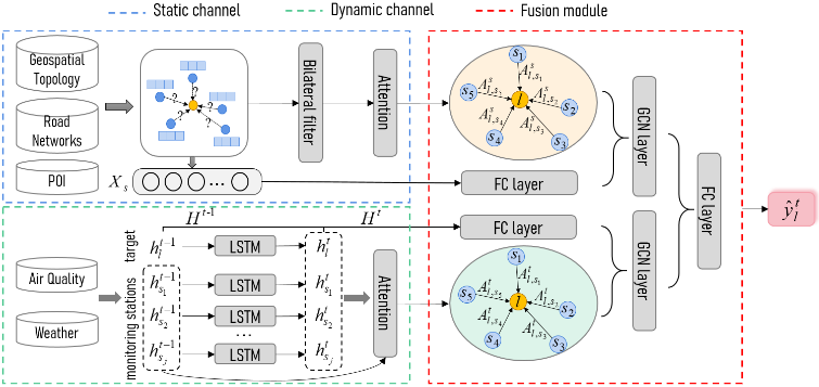
To model both static and dynamic spatial correlations, we first divide the features from multiple heterogeneous data sources into two categories.
Static geographic features. This set of features is derived from the geospatial topology and geo-context data of a target location and monitoring stations. We denote the static geographic features of all monitoring stations by Xs.
Dynamic spatial features. This set of features includes weather features and air quality features of a target location and monitoring stations. We denote weather features of target location l by lw, those of monitoring stations by Xw, and air quality features of monitoring stations by Xm. Note that in our problem target locations do not have air quality readings.
With the sets of static and dynamic features, we design a multi-channel attention model (MCAM), which consists of three major components, as illustrated in Figure 1. The first component is a static graph channel that learns the static spatial correlation from static geographic features. Unlike existing methods that either directly feed neighboring stations' static geographic features into DNNs or leverage attention mechanisms based on only Euclidean distance, the static graph channel combines the advantages of both an attention mechanism and graph-based modeling. Inspired by its use in image inpainting, bilateral filtering is used to better model the static spatial correlation by considering both the Euclidean distance and the similarity of geographic features between a target location and a station. The second component is a dynamic graph channel that captures the temporal evolutions of dynamic spatial features. We use LSTM networks to model the temporal evolutions of each monitoring station using both air quality data and weather data and the target location using only weather data. An attention mechanism is adopted to measure the extent of influence of a monitoring station on the target location at each time step. Two novel notions are introduced to more accurately measure the influence. The last component is the multi-channel graph convolutional fusion module that elegantly combines the graph and non-graph outputs from the two channels to make the final prediction.
4.2 Static Graph Channel Construction
We explicitly model the spatial influence of monitoring stations on a target location using a graph. Formally, given a target location l and a set of monitoring stations S, the output of the static graph channel is a weighted directed graph Gl = (Vl, El), where Vl = S ∪ {l} and (si, l) ∈ El indicates the static spatial influence of si ∈ S on l. Intuitively, modeling the static spatial influence of nearby monitoring stations on a target location without any air quality readings is similar to recovering a missing region in an image from its nearby pixels, where bilateral filters are a well-established solution. The general idea of bilateral filters is to replace the intensity of a pixel with a weighted average of intensity values from nearby pixels. A nice property is that the weights depend on not only Euclidean distances of pixels, but also other factors (e.g., radiometric differences). In image processing, the output of a classical bilateral filter [Tomasi and Manduchi, 1998] on a target pixel x, denoted by BF(x), is defined as follows:
where ξ is a nearby pixel, k-1 (x) is a normalization factor that ensures that pixel weights sum to 1.0, f(·) is an image function, c(ξ, x) is the geometric distance between ξ and x, and s(f(ξ), f(x)) is the photometric similarity between ξ and x (e.g., the similarity of color intensity). More specifically,
where d(ξ, x) is the Euclidean distance between ξ and x, and σd is a bilateral filtering parameter.
where δ(f(ξ), f(x)) is the similarity of the intensity values of ξ and x, and σr is another bilateral filtering parameter.
Since our goal is to learn different stations' static spatial influence on the target location, we employ an attention mechanism to quantify different stations' importance degree on the target location l. Here we design an adapted bilateral filtering score function for the attention mechanism as follows:
where d(si, l) is the Euclidean distance between si and l, ρ(si, l) is the Pearson correlation coefficient of the static geographic features of si and l, and the bilateral filtering parameters σd and σr are trainable parameters. Then the weight of
adjacency matrix As of the static spatial graph Gl for target location l. This graph does not change over time and will be used at each time step to fuse with the corresponding dynamic spatial graph to predict the air quality at location l.
4.3 Dynamic Graph Channel Construction
To capture the dynamic spatial correlation, we propose to model the temporal evolutions of dynamic spatial features and their interplay at each time step. Similarly, we would like to learn a weighted directed graph for target location l at time t, denoted by G t l = (S ∪ {l}, E t l ), where the weight of an edge (si, l) ∈ E t l gives the dynamic spatial influence of station si on l at time t. We use LSTM networks [Hochreiter and Schmidhuber, 1997] to model the temporal evolutions. An LSTMmaps an input sequence to an output sequence by an input gate unit, an output gate unit, a forget gate unit, and a more complex memory cell using the following equations:
where xt and ht are the input data and the corresponding hidden state at time t. f t , it and ot are the activation vectors of the forget gate, input gate and output gate, respectively. W ∈ Rh×d and b ∈ Rh are the weight matrices and bias parameters that need to be learned from the training data, where d and h are the input dimension and the number of hidden units, respectively. Note that we build an LSTM for each station and the target location. The input to a station's LSTM at time t, i.e., xt , is the concatenation of its air quality features and weather features, while the input to the target location's LSTM at time t only contains weather features as there is no air quality readings at the location. The initial inputs for monitoring stations and the target location are Xw‖Xm and lw (see Section 4.1), respectively, where ‖ means concatenation.
However, the hidden state ht of an LSTM only captures the temporal dependency of a station or the target location, and cannot directly reveal dynamic spatial correlations between them. Here we again employ attention mechanisms to learn the dynamic spatial correlation at each time step. However, designing the score function for dynamic spatial correlation needs special attention. We, for the first time, propose to use atmospheric dispersion theories to guide the design of the score function of the attention mechanism, and introduce two new notions, the atmospheric dispersion conditions and the hysteretic nature of air pollutant dispersion (i.e., the air quality of the target location is also affected by the air quality of stations in the previous time step as the dispersion process takes time). We first present the entire score function below, followed by its explanation:
where σ(·) is the ReLU activation function, the weight matrices Wh and Wa, vectors wd and bd are learnable model parameters. The weight matrices Wh and Wa help to balance the contributions of the hysteresis term and the atmospheric term. The effect of the hysteretic nature of a station si on l at time t is modeled by the hysteresis term FC(htsi , ht-1 si ). We use a simple fully connected neural network to learn the dependency between station si's hidden states htsi and ht-1 si at time t and time t-1, respectively. The impact of atmospheric dispersion conditions is modeled by the atmospheric term utsi ‖ vtsi ‖ angle(si,l). The horizontal wind velocity utsi , vertical wind velocity vtsi and the downwind relative angle between si and l are the most important atmospheric factors for air pollutant dispersion identified in well-established atmospheric dispersion models [Arystanbekova, 2004; Rakowska et al., 2014]. We combine all these features to learn the spatial influence of station si on l via a linear layer. With the above score function, we can calculate the weight of an edge (si, l)
are shared across all time steps. Similarly, all edge weights in G t l form its adjacency matrix At for l at time t.
4.4 Multi-Channel Graph Convolutional Fusion Network
With the adjacency matrices As and At learned from the static and dynamic channels, we fuse them along with other features to predict the target location l's air quality at time t via a multi-channel graph convolutional fusion network, as illustrated in Figure 1. Mathematically, the multi-channel graph convolutional fusion network is defined as follows:
where ˆ yt l is l's predicted air quality value at time t, σ(·) is the ReLU activation function, and Wf and bf are trainable parameters. AsFC (Xs)Ws fuses the graph and non-graph features from the static channel. Here Xs is the monitoring stations' static geographic features. A fully connected neural network is used to generate the embedding of Xs, and then As weights different dimensions in the embedding. Ws is a feature transformation matrix to learn. Similarly, AtFC (Ht ,Ht-1 ) Wt fuses the features from the dynamic channel. Ht and Ht-1 denote all monitoring stations' hidden states at time t and time t - 1, respectively. The fully connected neural network can also be considered as an embedding layer, whose output is weighted by At . Wt is another learnable feature transformation matrix. Finally, the features from the static and dynamic channels are concatenated and fused by a linear layer.
| PM2.5 | PM10 | NO2 | ||||
|---|---|---|---|---|---|---|
| MAE | RMSE | MAE | RMSE | MAE | RMSE | |
| KNN | 10.58/3.90 | 18.24/5.77 | 22.86/5.85 | 36.14/8.45 | 17.81/17.48 | 22.93/21.97 |
| LI | 10.66/3.33 | 19.30/5.11 | 21.08/5.37 | 33.74/7.89 | 17.29/20.03 | 21.99/25.45 |
| ADAIN | 8.28/2.02 | 15.06/3.11 | 14.88/2.73 | 24.55/4.62 | 6.91/6.11 | 9.84/8.40 |
| MCAM | 6.83/1.78 | 12.57/2.81 | 13.61/2.66 | 22.61/4.45 | 5.79/5.94 | 8.27/8.40 |
4.5 Model Learning
Since the fine-grained air quality inference problem is a regression problem, we consider the widely used loss function for regression tasks, namely the mean squared error (MSE). Formally, the objective function L we optimize is:
where M is the number of training instances, T is the prediction time window, xti is a training instance at time t, and Θ is the set of trainable parameters in the MCAMmodel. Since yt i is not available for a target location without a monitoring station, a common practice is to use some monitoring stations as target locations in training [Cheng et al., 2018].
5 Experiments
In this section, we empirically demonstrate the superior performance of MCAM on two benchmark real-word datasets.
5.1 Datasets andMetrics
For a fair comparison, we utilize the Beijing dataset, the only dataset used in the state-of-the-art solution [Cheng et al., 2018]. In addition, we use another London dataset to draw more convincing conclusions. Both datasets are widely used in extensive literature. We elaborate these two datasets below.
Air quality data. We collect air quality data, including air quality index (AQI), PM2.5, PM10, O3, NO2, CO, SO2, from all 35 ground-based air quality monitoring stations in Beijing 1 and PM2.5, PM10, and NO2 from all 13 ground-based monitoring stations in London 2 .
Meteorological data. For the Beijing dataset, we consider grid-based weather data from the Global Data Assimilation System (GDAS) 3 [Zhang et al., 2019]. Similar to [Zhang et al., 2019], we select five weather attributes: temperature, humidity, wind speed, and wind directions (including wind-u and wind-v in GDAS) and conduct a temporal linear interpolation to convert the 3-hourly raw data to hourly data. For the London dataset, its meteorological data has been preprocessed and is publically available 2 .
1 http://beijingair.sinaapp.com
2 https://github.com/for-competition/KDD CUP 2018
3 https://www.ncdc.noaa.gov/data-access/model-data/modeldatasets/global-data-assimilation-system-gdas
POIs. Similar to [Zheng et al., 2013], we consider 12 types of POIs from Amap of Beijing and London 4 , and compute the number of POIs in each category within the affecting region of a station or a target location as a feature.
Road networks. We download the road network data of Beijing and London from OpenStreetMap (OSM) 5 . There are five types of roads, and we calculate the number of each type of roads as a feature.
We process air quality data and meteorological data of Beijing from 01/01/2016 to 01/31/2018 and those of London from 01/01/2017 to 03/31/2018. The portions of training, validation, and test data are split by the ratio 8:1:1. The time window T is set to 12. Identical to [Cheng et al., 2018], we aim to predict the PM2.5, PM10 and NO2 values of a target location without monitoring stations at each time step during the time window. Since we only have ground truth for the locations with monitoring stations, similar to [Cheng et al., 2018], we randomly choose 3 out of the 35 monitoring stations in Beijing and 3 out of the 13 monitoring stations in London to be target locations. For each target location, we only use the remaining stations' air quality data to train a model so as to avoid data leakage.
We use two widely used evaluation metrics, mean absolute error (MAE) and root mean squared error (RMSE), to measure the performance of different prediction models.
5.2 Models
We compare MCAM with three representative competitors.
- k nearest neighbors (KNN) uses the average air pollutant value of the k closest monitoring stations as the prediction result. Identical to [Cheng et al., 2018], we set k = 3.
- Linear interpolation (LI) is a classical method that calculates a weighted average of PM2.5, PM10, or NO2 values of the monitoring stations [Cheng et al., 2018].
- ADAIN [Cheng et al., 2018] is the state-of-the-art method for fine-grained air quality prediction. We use the same hyperparameter setting reported in [Cheng et al., 2018].
We also summarize the hyperparameter setting of MCAM. We use 300 hidden units in an LSTM cell, and optimize the objective function using the Adam optimizer with learning rate 0.01. All fully connected neural networks have a single hidden layer with 200 neurons. We initialize all the model parameters from the uniform distribution between -0.1 and 0.1, and implement the model in PyTorch.
4 https://lbs.amap.com/api/webservice/download
5 https://www.openstreetmap.org/
| PM2.5 | PM10 | NO2 | ||||
|---|---|---|---|---|---|---|
| MAE | RMSE | MAE | RMSE | MAE | RMSE | |
| Distance | 7.70/2.08 | 13.72/3.34 | 15.33/3.26 | 25.01/5.35 | 6.76/6.79 | 9.61/9.42 |
| BF | 6.83/1.78 | 12.57/2.81 | 13.61/2.66 | 22.61/4.45 | 5.79/5.94 | 8.27/8.40 |
| PM2.5 | PM10 | NO2 | ||||
|---|---|---|---|---|---|---|
| MAE | RMSE | MAE | RMSE | MAE | RMSE | |
| MCAM-h | 8.12/2.11 | 14.91/3.39 | 14.79/3.32 | 25.10/5.08 | 7.29/6.51 | 10.34/8.85 |
| MCAM-a | 8.26/1.97 | 15.05/3.12 | 14.27/2.91 | 23.85/4.87 | 5.99/6.35 | 8.67/9.09 |
| MCAM-sc | 7.46/2.11 | 13.15/3.39 | 14.35/3.15 | 24.07/5.16 | 6.56/6.44 | 9.43/9.09 |
| MCAM-dc | 21.14/6.51 | 35.85/11.30 | 30.87/9.06 | 49.83/13.77 | 8.92/18.04 | 12.47/22.90 |
| MCAM | 6.83/1.78 | 12.57/2.81 | 13.61/2.66 | 22.61/4.45 | 5.79/5.94 | 8.27/8.40 |
5.3 Experimental Results
Performance comparison. We report the main experimental results in Table 1. It can be seen that MCAM obtains the best performance in all settings on both datasets. Simple models, such as KNN and LI, are not able to achieve meaningful accuracy, validating the technical challenge of finegrained air quality inference. Compared to the state-of-theart model ADAIN, MCAM's performance improvements are up to 17.5% in terms of MAE and 16.5% in terms of RMSE on the Beijing dataset, and up to 11.8% in terms of MAE and 9.7% in terms of RMSE on the London dataset. We believe that this is due to a more comprehensive modeling of dynamic spatial correlations and a more effective fusion between static and dynamic correlations. The improvements on the London dataset are smaller because the monitoring stations are within a smaller region, making it relatively easier to predict.
Effect of bilateral-filtering-based attention. We design an adapted bilateral filtering technique as the basis for integrating multiple factors in the attention mechanism. To prove its effectiveness, we consider an alternative that employs a distance-based attention mechanism. We denote the bilateralfiltering-based attention mechanism by BF and the alternative by Distance. The results are presented in Table 2. As can be observed, BF achieves consistently better performance in all settings. On the Beijing dataset, in which the monitoring stations are far apart, considering both Euclidean distances and the similarity of geographic features is more rewarding.
Effects of other key components. In the last set of experiments, we demonstrate the benefits of the two graph channels, hysteresis item and the atmospheric item. We construct a variant without the hysteresis item (MCAM-h), a variant without the atmospheric item (MCAM-a), a variant without the static graph channel (MCAM-sc), and a variant without the dynamic graph channel (MCAM-dc). The experimental results are given in Table 3. It can be observed that both terms can bring performance improvements. On the Beijing dataset, which represents a more challenging task, the improvements are more obvious. Although the benefit of having the static graph channel is clear, it is a bit surprising to see that the two terms are even more important than the static graph channel. Arguably, the dynamic graph channel is the most important component of MCAM. This result is well aligned with our motivation that fully modeling dynamic spatial correlations is key to fine-grained air quality inference.
6 Conclusion
In this paper, we studied the practical problem of fine-grained air quality inference. In view of existing studies' insufficient attention on dynamic spatial correlation, we proposed the novel MCAM model that explicitly models static and dynamic spatial correlations between a target location and monitoring stations as two separate channels. In the static graph channel, we designed a bilateral filtering-based attention layer to capture the static spatial correlation as a graph; in the dynamic graph channel, we proposed to use LTSM networks to model the temporal evolutions of monitoring stations and a target location. The hysteresis term and the atmospheric term were introduced to better measure the spatial correlation at each time step. A multi-channel graph convolutional fusion network was also devised to fuse the graph and non-graph features from both channels. Our comprehensive experimental results validate MCAM's superiority.
Acknowledgements
This work was supported by the National Key R&D Program of China under Grant No. 2020YFB1710200, the National Natural Science Foundation of China under Grant No. 61872105 and No. 62072136, the Fundamental Research Funds for the Central Universities under Grant No. 3072020CFT2402 and No. 3072020CFT0603, and the Opening Fund of Acoustics Science and Technology Laboratory under Grant No. SSKF2020003.
@inproceedings{ijcai2021p346,
  title     = {Fine-Grained Air Quality Inference via Multi-Channel Attention Model},
  author    = {Han, Qilong and Lu, Dan and Chen, Rui},
  booktitle = {Proceedings of the Thirtieth International Joint Conference on
               Artificial Intelligence, {IJCAI-21}},
  publisher = {International Joint Conferences on Artificial Intelligence Organization},
  editor    = {Zhi-Hua Zhou},
  pages     = {2512--2518},
  year      = {2021},
  month     = {8},
  note      = {Main Track},
  doi       = {10.24963/ijcai.2021/346},
  url       = {https://doi.org/10.24963/ijcai.2021/346},
}
TY - CPAPER TI - Fine-Grained Air Quality Inference via Multi-Channel Attention Model AU - Han, Qilong AU - Lu, Dan AU - Chen, Rui T2 - Proceedings of the Thirtieth International Joint Conference on Artificial Intelligence, IJCAI-21 PB - International Joint Conferences on Artificial Intelligence Organization PY - 2021 SP - 2512 EP - 2518 DO - 10.24963/ijcai.2021/346 UR - https://doi.org/10.24963/ijcai.2021/346 ER -Copied
Machine-readable versions of this paper, for tools and AI agents:





