
Riemannian Stochastic Recursive Momentum Method for non-Convex Optimization
Proceedings of the Thirtieth International Joint Conference on Artificial Intelligence. Main Track. Pages 2505-2511.
https://doi.org/10.24963/ijcai.2021/345
Keywords
- Machine Learning: Online Learning
Abstract
We propose a stochastic recursive momentum method for Riemannian non-convex optimization that achieves a nearly-optimal complexity to find epsilon-approximate solution with one sample. The new algorithm requires one-sample gradient evaluations per iteration and does not require restarting with a large batch gradient, which is commonly used to obtain a faster rate. Extensive experiment results demonstrate the superiority of the proposed algorithm. Extensions to nonsmooth and constrained optimization settings are also discussed.
- [Arjevani et al., 2019] Yossi Arjevani, Yair Carmon, John C Duchi, Dylan J Foster, Nathan Srebro, and Blake Wood- worth. Lower bounds for non-convex stochastic optimiza- tion. arXiv:1912.02365, 2019.
- [Bécigneul and Ganea, 2018] Gary Bécigneul and Octavian- Eugen Ganea. Riemannian adaptive optimization methods. arXiv:1810.00760, 2018.
- [Bonnabel, 2013] Silvere Bonnabel. Stochastic gradient de- scent on riemannian manifolds. Transactions on Auto- matic Control, 58(9):2217-2229, 2013.
- [Chang and Lin, 2011] Chih-Chung Chang and Chih-Jen Lin. LIBSVM: A library for support vector machines. ACM Transactions on Intelligent Systems and Technology, 2(3):1-27, 2011.
- [Cheng et al., 2012] Guang Cheng, Hesamoddin Salehian, and Baba C Vemuri. Efficient recursive algorithms for computing the mean diffusion tensor and applications to dti segmentation. In European Conference on Computer Vision, pages 390-401. Springer, 2012.
- [Cutkosky and Orabona, 2019] Ashok Cutkosky and Francesco Orabona. Momentum-based variance reduction in non-convex sgd. In Advances in Neural Information Processing Systems, pages 15236-15245, 2019.
- [Han and Gao, 2020] Andi Han and Junbin Gao. Variance reduction for riemannian non-convex optimization with batch size adaptation. arXiv:2007.01494, 2020.
- [Hosseini and Sra, 2017] Reshad Hosseini and Suvrit Sra. An alternative to em for Gaussian mixture mod- els: Batch and stochastic Riemannian optimization. arXiv:1706.03267, 2017.
- [Iannazzo and Porcelli, 2018] Bruno Iannazzo and Margherita Porcelli. The Riemannian Barzilai-Borwein method with nonmonotone line search and the matrix geometric mean computation. IMA Journal of Numerical Analysis, 38(1):495-517, 2018.
- [Ji et al., 2019] Kaiyi Ji, Zhe Wang, Bowen Weng, Yi Zhou, Wei Zhang, and Yingbin Liang. History-gradient aided batch size adaptation for variance reduced algorithms. arXiv:1910.09670, 2019.
- [Kasai et al., 2018] Hiroyuki Kasai, Hiroyuki Sato, and Bamdev Mishra. Riemannian stochastic recursive gradi- ent algorithm. In International Conference on Machine Learning, pages 2516-2524, 2018.
- [Kasai et al., 2019] Hiroyuki Kasai, Pratik Jawanpuria, and Bamdev Mishra. Riemannian adaptive stochastic gradient algorithms on matrix manifolds. arXiv:1902.01144, 2019.
- [Kingma and Ba, 2014] Diederik P Kingma and Jimmy Ba. Adam: A method for stochastic optimization. arXiv:1412.6980, 2014.
- [Krizhevsky et al., 2009] Alex Krizhevsky, Geoffrey Hinton, et al. Learning multiple layers of features from tiny im- ages. 2009. [Kylberg, 2014]
- G Kylberg. The kylberg texture dataset v. 1.0. external report (blue series) 35, centre for image anal- ysis, swedish university of agricultural sciences and upp- sala university, uppsala, sweden (2011). 2014.
- [LeCun et al., 1998] Yann LeCun, Léon Bottou, Yoshua Bengio, and Patrick Haffner. Gradient-based learning ap- plied to document recognition. Proceedings of the IEEE, 86(11):2278-2324, 1998.
- [Li et al., 2020] Jun Li, Li Fuxin, and Sinisa Todorovic. Effi- cient Riemannian optimization on the Stiefel manifold via the Cayley transform. arXiv:2002.01113, 2020.
- [Meghwanshi et al., 2018] Mayank Meghwanshi, Pratik Jawanpuria, Anoop Kunchukuttan, Hiroyuki Kasai, and Bamdev Mishra. Mctorch, a manifold optimization library for deep learning. arXiv:1810.01811, 2018.
- [Nene et al., 1996] Sameer A Nene, Shree K Nayar, Hiroshi Murase, et al. Columbia object image library (coil-100). 1996.
- [Robbins and Monro, 1951] Herbert Robbins and Sutton Monro. A stochastic approximation method. The Annals of Mathematical Statistics, pages 400-407, 1951.
- [Roy et al., 2018] Soumava Kumar Roy, Zakaria Mhammedi, and Mehrtash Harandi. Geometry aware constrained optimization techniques for deep learning. In Conference on Computer Vision and Pattern Recognition, pages 4460-4469, 2018.
- [Sato et al., 2019] Hiroyuki Sato, Hiroyuki Kasai, and Bamdev Mishra. Riemannian stochastic variance reduced gradient algorithm with retraction and vector transport. SIAM Journal on Optimization, 29(2):1444-1472, 2019.
- [Staib et al., 2019] Matthew Staib, Sashank J Reddi, Satyen Kale, Sanjiv Kumar, and Suvrit Sra. Escaping saddle points with adaptive gradient methods. arXiv:1901.09149, 2019.
- [Theis et al., 2009] Fabian J Theis, Thomas P Cason, and P- A Absil. Soft dimension reduction for ica by joint diag- onalization on the stiefel manifold. In International Con- ference on Independent Component Analysis and Signal Separation, pages 354-361. Springer, 2009.
- [Tieleman and Hinton, 2012] Tijmen Tieleman and Geoffrey Hinton. Lecture 6.5-rmsprop: Divide the gradient by a running average of its recent magnitude. COURSERA: Neural Networks for Machine Learning, 4(2):26-31, 2012.
- [Tran-Dinh et al., 2019] Quoc Tran-Dinh, Nhan H Pham, Dzung T Phan, and Lam M Nguyen. Hybrid stochastic gradient descent algorithms for stochastic nonconvex opti- mization. arXiv:1905.05920, 2019.
- [Wright et al., 2008] John Wright, Allen Y Yang, Arvind Ganesh, S Shankar Sastry, and Yi Ma. Robust face recog- nition via sparse representation. Transactions on Pattern Analysis and Machine Intelligence, 31(2):210-227, 2008.
- [Zhou et al., 2019] Pan Zhou, Xiaotong Yuan, Shuicheng Yan, and Jiashi Feng. Faster first-order methods for stochastic non-convex optimization on Riemannian man- ifolds. arXiv:1811.08109, 2019.
References were extracted automatically from the PDF and may contain errors.
Full text extracted automatically from the PDF; figures, tables and equations may differ. The PDF is the version of record.
1 Introduction
We consider the problem of expectation (online) minimization over a Riemannian manifold M:
where F: M -→ R is a sufficiently smooth and potentially non-convex function. When ω can be finitely sampled from its support Ω, problem (1) reduces to empirical risk (finitesum) minimization, minx∈MF(x) := 1n ∑ni=1 fi(x), where n is the number of component functions.
In this paper, we focus on the case where full gradient of F(x) is inaccessible as in online setting or when n is extremely large under finite-sum setting. Riemannian optimization is ubiquitous in a variety of contexts. For example, principal component analysis (PCA) and matrix completion can be formulated on Grassmann manifold [Kasai et al., 2018]. In image processing, the tasks of diffusion tensor imaging segmentation and clustering can be cast on symmetric positive definite (SPD) manifold [Cheng et al., 2012]. Joint diagonalization for independent component analysis (ICA) is a problem over Stiefel manifold, which is useful for signal separation [Theis et al., 2009].
Riemannian geometry provides the minimal ingredients that allow unconstrained optimization methods to be properly defined. A default solver to problem (1) is Riemannian stochastic gradient descent (RSGD) [Bonnabel, 2013], which is a generalization of classic SGD [Robbins and Monro, 1951]. Recently, SGD with coordinate-wise adaptive learning rates has become predominately popular within Deep Learning community, such as RMSProp [Tieleman and Hinton,
2012] and Adam [Kingma and Ba, 2014]. These variants have been proved to improve robustness and escape saddle points faster [Staib et al., 2019]. Under Riemannian optimization, the lack of a canonical coordinate system and the highly nonlinear geometry make it difficult to extend such adaptation effectively. Regardless, Roy et al. (2018) proposed constrained SGD with momentum (cSGD-M) and constrained RMSProp (cRMSProp) that adapt learning rates by coordinate-wise operations on matrix manifolds. However unlike Euclidean space, parallelly transporting past gradients will likely distort gradient features, such as sparsity. Also, no convergence guarantee has been provided. B´ecigneul and Ganea (2018) generalized Adam-like adaptation and momentum to a product of Riemannian manifolds (referred to as RADAM and RAMSGRAD). Li et al. (2020) introduced Cayley-Adam tailored for Stiefel manifold, exploiting its unique geometry. The only work that proves non-convex convergence on matrix manifolds is [Kasai et al., 2019], where they proposed RASA that adapts row and column subspaces of underlying manifold, ensuring a convergence rate of ˜ O(1/√T ). This matches that of RSGD up to a logarithmic factor.
Although SGD-based methods enjoy low sampling cost, i.e. O(1) per iteration (one-sample), the main bottleneck that slows down convergence is the unvanished gradient variance. For this problem, variance reduction (VR) techniques are gaining increasing attention. Many methods, including Riemannian stochastic variance reduced gradient (RSVRG) [Sato et al., 2019], stochastic recursive gradient (RSRG) [Kasai et al., 2018], stochastic path-integrated differential estimator (RSPIDER) [Zhou et al., 2019] are generalized from their Euclidean versions. The main idea is to correct for stochastic gradient deviation by periodically computing a large batch gradient. As a result, gradient variance decreases as training progresses. Besides finite-sum optimization, Riemannian VRs also enjoy favourable complexity under online setting [Zhou et al., 2019; Han and Gao, 2020]. Specifically, RSVRG requires O(ϵ-10/3 ) stochastic gradient queries to return an ϵ-approximate solution (see Definition 1), which improves on O(ϵ-4 ) of RSGD. RSRG and RSPIDER require an even lower complexity of O(ϵ-3 ). This rate has been proved to be optimal for stochastic optimization on Euclidean space under an additional mean-squared smoothness assumption [Arjevani et al., 2019].
Nevertheless, these online VR methods still require computing a large batch gradient, i.e. O(ϵ-2 ), for each epoch and the mini-batch size for each inner iteration should also be at least O(ϵ-1 ). Therefore, we introduce a novel online variance reduction method, inspired by a recently proposed recursive momentum estimator [Cutkosky and Orabona, 2019]. Our contributions are summarized below.
| Complexity | Large Batch | Small Batch | Restarting | Manifold types | |
|---|---|---|---|---|---|
| RSRG/RSPIDER [Han and Gao, 2020; Zhou et al., 2019] | O(ϵ-3 ) | O(ϵ-2 ) | O(ϵ-1 ) | Yes | General |
| RSGD [Hosseini and Sra, 2017] | O(ϵ-4 ) | - | O(1) | No | General |
| RASA [Kasai et al., 2019] | ˜ O(ϵ-4 ) | - | O(1) | No | Matrix manifolds |
| RSRM (this work) | ˜ O(ϵ-3 ) | O(1) | O(1) | No | General |
- We propose a Riemannian stochastic recursive momentum (RSRM) method that achieves a gradient complexity of ˜ O(ϵ-3 ) for online non-convex optimization, matching the lower bound up to a logarithmic factor.
- RSRM requires only O(1) gradient computations per iteration and does not need restarting with a large batch gradient. Thus, our method preserves the efficiency of SGD while achieving fast convergence as VR methods.
- Our convergence result holds for general manifolds while other online adaptive methods apply to restricted manifold types, such as matrix manifolds [Roy et al., 2018; Kasai et al., 2019], product manifolds [B´ecigneul and Ganea, 2018] and Stiefel manifold [Li et al., 2020].
- Our algorithm does not adapt learning rate as in [Cutkosky and Orabona, 2019], therefore resulting in a simplified convergence analysis that does not need gradient Lipschitz assumption. This also benefits practical implementation by reducing the number of hyperparameters. Extensive experiments confirm that our method significantly outperforms other one-sample methods.
The rest of this paper is organized as follows. Section 2 introduces some useful definitions, notations and assumptions used for convergence analysis. Section 3 describes our proposed algorithm and highlights its relations with RSGD, variance reduction and stochastic momentum. Section 4 presents convergence analysis for RSRM and Section 5 evaluates the proposed method on a variety of tasks and manifolds.
2 Preliminaries
Riemannian manifold is a manifold with a smooth inner product 〈·, ·〉x : TxM× TxM -→ R defined on tangent space TxM for every x ∈ M. The induced norm on TxM is ‖u‖x := √〈u, u〉x. Retraction Rx : TxM -→ M maps a tangent vector to manifold surface satisfying Rx(0) = x and DRx(0)[u] = u. The retraction curve is defined as c(t) := Rx(tξ) for ξ ∈ TxM. Denote y = Rx(ξ). Then vector transport T y x (or equivalently Tξ) with respect to retraction R maps u ∈ TxM to T y x u ∈ TyM along the defined retraction curve c(t). Exponential map Expx is a special instance of retraction by restricting retraction curve to be a geodesic. Similarly, as a special case of vector transport, parallel transport P y x transports a tangent vector in 'parallel' while preserving its norm and direction. In this paper, we consider the more general and computationally efficient retraction and vector transport. Therefore our results can be trivially applied to exponential map and parallel transport (See Appendix). Implicitly, we consider only isometric vector transport T y x , which satisfies 〈u, v〉x = 〈T y x u, T y x v〉y for all u, v ∈ TxM.
Notations. For the discussions that follow, we omit the subscript for norm and inner product, which should be clear from the contexts. We define a sampling set S = {ω1, ..., ω|S|} with cardinality |S|. Each ω(·) is sampled independently from Ω. We thus denote the Riemannian stochastic gradient gradfS(x) := 1 |S| ∑ω∈S gradf(x, ω) ∈ TxM. We denote g(t) = O(h(t)) if there exists a positive constant M and t0 such that g(t) ≤ Mh(t) for all t ≥ t0. We use ˜ O(·) to further hide poly-logarithmic factors. We refer to ‖ · ‖ as the induced norm on tangent space of Riemannian manifold. Now we are ready to make some assumptions as follows.
Assumption 1. Iterates generated by RSRM stay continuously in a neighbourhood X ⊆ M that contains an optimal point x∗ . The objective F is continuously differentiable and has bounded suboptimality. That is, for all x ∈ X, F (x) - F (x∗ ) ≤ ∆, with ∆ ≥ 0.
Assumption 2. Stochastic gradient gradf(x, ω) is unbiased and has bounded variance. That is, for all x ∈ X, ω ∈ Ω, it satisfies thatEωgradf(x, ω) = gradF(x), and
Assumption 3. The objective F is retraction L-smooth with respect to retraction R. That is, there exists a positive constant L such that for all x, y = Rx(ξ) ∈ X , we have
These three assumptions are standard in Riemannian stochastic gradient methods [Hosseini and Sra, 2017; Kasai et al., 2018]. Note that the assumption of bounded iterates in neighbourhood X can be made with respect to the entire manifoldM, which results in stricter conditions on the retraction and vector transport in the following assumptions. To ensure retraction L-smoothness as in Assumption 3, we require an upper-bounded Hessian property on the pullback function F ◦R : TxM -→ R. That is, for all x ∈ X and u ∈ TxMwith unit norm, d2F(Rx(tu)) dt2 ≤ L. In the work of RASA [Kasai et al., 2019], the variance bound in Assumption 2 is replaced by G-gradient Lipschitz, which requires ‖gradf (x, ω)‖ ≤ G. This, however, amounts to a stronger assumption.
According to [Arjevani et al., 2019], under the first three assumptions, SGD is minimax optimal. To obtain faster convergence, one further assumption of mean-squared retraction Lipschitz is required. This assumption is a straightforward generalization of mean-squared Lipschitz on Euclidean space, which is the minimal additional requirement to achieve the complexity lower bound.
Assumption 4. The objective F is mean-squared retraction ˜L Lipschitz. That is, there exists a positive constant ˜L such that for all x, y = Rx(ξ) ∈ X , ω ∈ Ω,
holds with vector transport T y x along the retraction curve c(t) := Rx(tξ).
Note that the standard assumption of retraction Lipschitzness is made with respect to parallel transport and one additional assumption that bounds the difference between vector transport and parallel transport is needed for Assumption 4 to hold [Han and Gao, 2020]. In this work, algorithm complexity is measured by the number of stochastic first order oracles to achieve ϵ-approximate solution, defined as follows.
Definition 1 (ϵ-approximate solution and SFO). ϵapproximate solution by a stochastic algorithm is an output x such that E‖gradF(x)‖2 ≤ ϵ2 . One stochastic firstorder oracle (SFO) outputs a stochastic gradient gradf(x, ω) given inputs x and ω drawn from Ω.
3 Algorithms
3.1 RSGD-Variance Reduction andMomentum
Riemannian stochastic gradient makes the following retraction update: xt+1 = Rxt (-ηtgradfSt (xt)). This allows updates to follow the negative gradient direction while staying on the manifold. Variance reduction techniques utilize past gradient information to construct a modified gradient estimator with decreasing variance. In particular, the recursive gradient estimator in RSRG/RSPIDER achieves the optimal rate of O(ϵ-3 ). That is, for each outer loop, a large batch gradient is computed as d0 = gradfS0 (x0), where |S0| is set to n under finite-sum setting and O(ϵ-2 ) under online setting. Within each inner iteration, stochastic gradient is corrected recursively based on its previous iterate:
where vector transport T xt xt-1 is necessary to relate gradients on disjoint tangent spaces. To achieve the optimal complexity, mini-batch size |St| is set to be at least O(ϵ-1 ). This choice of batch size can become very large, especially when we desire more accurate solutions.
On the other hand, stochastic gradient with momentum is not new on Euclidean space, while the first paper that presents such an idea on Riemannian manifold is [Roy et al., 2018].
Algorithm 1 Riemannian SRM
- 1: Input: Step size ηt, recursive momentum parameter ρt, Initial point x1.
- 2: Compute d1 = gradfS1 (x1).
- 3: for t = 1, ..., T do
- 4: Update xt+1 = Rxt (-ηtdt).
- 5: Compute dt+1 = gradfSt+1 (xt+1) + (1 - ρt+1)T xt+1 xt (dt -gradfSt+1 (xt)).
- 6: end for
- 7: Output: ˜x uniformly chosen at random from {xt}Tt=1 .
They simply take a combination of current stochastic gradient and transported momentum, given as
where ρt is commonly set to be 0.9. This idea has then been used in generalizing Adam and AMSGrad to Riemannian optimization [B´ecigneul and Ganea, 2018], where they only established convergence on a product of manifolds for geodesically convex functions. Even on Euclidean space, the effectiveness of stochastic momentum over vanilla SGD has remained an open question.
3.2 Proposed RSRM
Our proposed RSRM is given in Algorithm 1 where we extend the recursive momentum estimator, originally introduced in [Cutkosky and Orabona, 2019; Tran-Dinh et al., 2019]:
which hybrids stochastic gradient with the recursive gradient estimator in (2) for ρt ∈ [0, 1]. This can be also viewed as combining momentum estimator in (3) with a scaled difference of gradfSt (xt) - T xt xt-1 gradfSt (xt-1). Note that we recover vanilla RSGD when ρt = 1 and the recursive estimator in (2) when ρt = 0. As we will demonstrate in Section 4, ρt should be decreasing rather than fixed, thereby enabling a smooth transition from RSGD to RSRG. As a result, we do not require restarting the algorithm to achieve the optimal convergence. One remark is that the idea of transition from SGD to VR also appears in many batch size adaptation strategies [Ji et al., 2019; Han and Gao, 2020].
Compared with algorithm designs in Euclidean versions of SRM [Cutkosky and Orabona, 2019; Tran-Dinh et al., 2019], our formulation and parameter settings are largely different. Specifically, Cutkosky and Orabona (2019) further adapt the recursive momentum parameter ρt to the learning rate ηt where the latter itself is adapted to the norm of stochastic gradient. This is claimed to relieve the parameter tuning process. However, they reintroduce three parameters, which are even less intuitive to be tuned (even though some are fixed to a default value). As shown in Section 4, we only require tuning the initial step size η0 and initial momentum parameter ρ0 (where the latter can be fixed to a good default value). Furthermore, the adaptive step size requires a uniform gradient Lipschitz condition, the same as in [Kasai et al., 2019]
and also a uniform smoothness assumption, which is stronger than mean-squared smoothness in our setting. On the other hand, Tran-Dinh et al. (2019) replaces gradfSt (xt) in (4) with gradfBt (xt) where Bt is independent of St. This increases sampling complexity per iteration and also complicates its convergence analysis. In addition, they still require a large initial batch size |S0| = O(ϵ-1 ) while our |S0| = O(1).
4 Convergence Results
In this section, we prove convergence of RSRM. We first present a Lemma that bounds the estimation error of the recursive momentum estimator.
Lemma 1 (Estimation error bound). Suppose Assumptions 1 to 4 hold and consider Algorithm 1. Then we have
The proof of this Lemma can be found in Appendix where it follows an idea similar to the bound in RSRG/RSPIDER [Han and Gao, 2020]. The key difference is that we further use E‖dt‖2 ≤ 2E‖dt - gradF(xt)‖2 + 2E‖gradF(xt)‖2 to show dependence on the full gradient. Based on the claims in [Cutkosky and Orabona, 2019], we consider ρt = O(t-2/3 ) and ηt = O(t-1/3 ), so that E‖dt+1 - gradF(xt+1)‖2 = O(t-2/3 + E‖gradF(xt)‖2 ). To see this, denote st+1 = dt+1-gradF(xt+1). Then by noting that (1-ρt)2 ≤ 1-ρt ≤ 1 and η2 t ≤ ηt ≤ 1, Lemma 1 suggests that E‖st+1‖2 ≤ O(1-t-2/3 )E‖st‖2 +O(t-2/3 )E‖gradF (xt)‖2 +O(t-4/3 ). Simply setting E‖st+1‖2 = E‖st‖2 yields the result. This implies that E‖gradF(xt)‖2 = O(T -2/3 ), which matches the optimal rate of convergence. This claim is stated formally in the following Theorem. For simplicity, we consider |St| = b for all t.
Theorem 1 (Convergence and complexity of RSRM). Suppose Assumptions 1 to 4 hold and consider Algorithm 1 with ηt = cη(t + 1)-1/3 , ρt = cρt-2/3 where cη ≤ 1L and cρ = ( 10˜L2 b + 13 )c2η . Then we have
withM := (6∆+ σ2 2˜L2 + σ2 ln(T+1) ˜L2 )/cη. To get ϵ-approximate solution, we require an SFO complexity of ˜ O(ϵ-3 ).
Theorem 1 claims that RSRM achieves a nearly-optimal complexity of ˜ O(ϵ-3 ) with one-sample gradient, i.e. b = O(1). And specifically under noiseless case where σ2 = 0, we can further improve this result to the lower bound complexity O(ϵ-3 ). One final remark can be made that our step size decays at a rate of O(t-1/3 ), which is slower compared to the SGD-based rate of O(t-1/2 ). This step size sequence is crucial for achieving the faster convergence, coupled with gradually reduced variance.
5 Experiments
In this section, we compare our proposed RSRM with other one-sample online methods. The benchmark is the standard RSGD [Bonnabel, 2013]. We also consider cSGD-M and cRMSProp [Roy et al., 2018] where past gradients are transported by a vector transport operator. For cRMSProp, we do not project and vector-transport its adaptation term, which is an element-wise square of stochastic gradient. Instead, we treat it as an element in the ambient Euclidean space and therefore only project the resulting scaled gradient after applying this term. This modification yields the full-matrix version of the vectorized variant of RASA and turns out to significantly outperform its original design. Also we compare with RAMSGRAD [B´ecigneul and Ganea, 2018], which is designed for product manifolds. We thus modify the gradient momentum similar as in [Roy et al., 2018] while accumulating square norm of gradient instead of element-wise square. Hence, it only adapts the step size rather than the gradient. Finally, we consider RASA [Kasai et al., 2019] that adapts column and row subspaces of matrix manifolds. We similarly label its variants as RASA-L, RASA-R and RASA-LR to respectively represent adapting row (left) subspace, column (right) subspace and both.
All methods start with the same initialization and terminate when the maximum iteration number is reached. For competing methods, we consider a square-root decaying step size ηt = η0t-1/2 , suggested in [Kasai et al., 2019]. We set the parameters of RSRM according to the theory, i.e. ηt = η0t-1/3 and ρt = ρ0t-2/3 . A default value of ρ0 = 0.1 provides good empirical performance. For all methods, η0 are selected from {1, 0.5, 0.1, ..., 0.005, 0.001}. The gradient momentum parameter in cSGD-M and RAMSGRAD is set to be 0.9 and the adaptation momentum parameter in cRMSProp, RAMSGRAD and RASA is set to be 0.999. We choose a mini-batch size of 5 for RSRM and 10 for all other algorithms to ensure an identical per-iteration cost of gradient evaluation. The initial batch size for RSRM is fixed to be 100 (except for the problem of ICA where it is set to be 200). All algorithms are coded in Matlab and experiments are conducted on a laptop with a i5-8600 3.1GHz CPU processor.
We consider principal component analysis (PCA) on Grassmann manifold, joint diagonalization of independent component analysis (ICA) on Stiefel manifold and computing Riemannian centroid (RC) on SPD manifold. Stiefel manifold St(r, d) = {X ∈ Rd×r : XT X = Ir} is defined as the set of d × r column orthonormal matrices, which is a natural embedded submanifold of Rd×r . Grassmann manifold G(r, d) is the set of r-dimensional subspaces in Rd . One representation of Grassmann manifold is by a Stiefel matrix X ∈ Rd×r with orthonormal columns that span the subspace. This representation is not unique. Indeed, any XR for R ∈ O(r) is equivalent to X, where O(r) is the orthogonal group of dimension r. Hence, Grassmann manifold can be viewed as a quotient of Stiefel manifold, written as St(r, d)/O(r). Finally, SPD manifold S d++ is the set of d×d symmetric positive definite matrices, which forms the interior of a convex cone embedded in Rd(d+1)/2 . Manifold retractions and vector transports used in the following experiments are discussed in Appendix.
5.1 PCA on GrassmannManifold
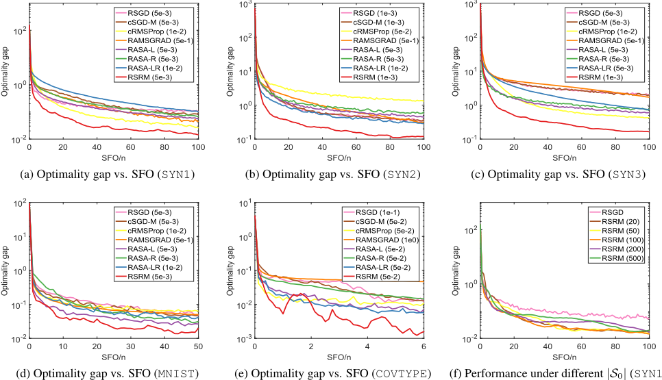
Consider n samples, represented by xi ∈ Rd , i = 1, ..., n. PCA aims to find a subspace where projection onto this subspace minimizes reconstruction error. This defines a problem on Grassmann manifold, written as minU∈G(r,d) 1n ∑ni=1 ‖xi -UUT xi‖2 . We first test RSRM on a baseline synthetic dataset (SYN1) with (n, d, r) = (104 , 102 , 10). Then we increase dimension to 500 (SYN2) and consider a higher rank case with r = 20 (SYN3). In addition, we consider two empirical datasets, MNIST [LeCun et al., 1998] with (n, d, r) = (60000, 784, 10) and COVTYPE from LibSVM [Chang and Lin, 2011] with (n, d, r) = (581012, 54, 10). We measure performance in terms of the difference between current function value to the minimum, pre-calculated using Matlab function PCA. Convergence results and the best-tuned η0 are shown in Figure 1. We find that RSRM consistently outperforms others on every dataset (Figure 1(a) to 1(e)). It is also observed that on 'easy' datasets, such as SYN1 and SYN2, adaptive methods perform similarly compared with well-tuned SGD whereas RSRM demonstrates its clear advantage. Figure 1(f) shows that RSRM seems to be insensitive to the initial batch size and surprisingly, larger batch size provides no benefit for this problem.
5.2 ICA on Stiefel Manifold
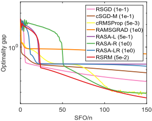
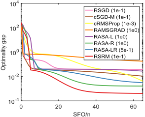
ICA (or blind source separation) aims to recover underlying components of observed multivariate data by assuming mutual independence of source signals. Joint diagonalization is a useful pre-processing step that searches for a pseudoorthogonal matrix (i.e. Stiefel matrix) [Theis et al., 2009] by solving minU∈St(r,d) - 1n ∑ni=1 ‖diag(UT XiU)‖2F with diag(A) returning diagonal elements of matrix A. The symmetric matrices Xi ∈ Rd×d can be time-lagged covariance matrices or cumulant matrices constructed from the observed signals. We consider three image datasets described as follows. YALEB [Wright et al., 2008] collects n = 2414 face images taken from various lighting environments. CIFAR100 [Krizhevsky et al., 2009] contains n = 60000 images of 100 objects and COIL100 [Nene et al., 1996] is made up of n = 7200 images from 100 classes. To construct covariance representations from these datasets, we first downsize each image to 32×32 before applying Gabor-based kernel to extract Gabor features. Then the feature information is fused in a region covariance descriptors of size 43×43. We choose r = d = 43 for all problems and the results are presented in Figure 2. Optimal solution is obtained by running RSRM for sufficiently long. Similarly, we find that RSRM, although showing slow progress at the initial epochs, quickly converges to a lower value compared with others. This is mainly attributed to its variance reduction nature.
5.3 RC on SPDManifold
(b) Optimality gap vs. SFO (CIFAR100)
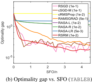
5.4 Additional Experiment Results
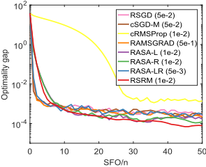
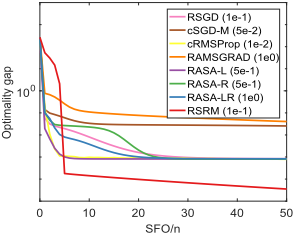
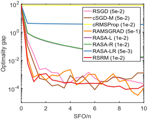
Computing Riemannian centroid on SPD manifold S d++ are fundamental in many computer vision tasks [Cheng et al., 2012]. The problem concerns finding a mean representation of a set of SPD matrices, Xi. The geodesic distance on S d++ induced by Affine Invariant Riemannian Metric (AIRM) is d2 (X1,X2) = ‖ log(X-1/2 1 X2X-1/2 1 )‖2F where log(·) is the principal matrix logarithm. Riemannian centroid with respect to this distance is obtained by solving minC∈S d++ 1n ∑ni=1 d2 (C, Xi). We first consider a simulated dataset consisting of n = 5000 SPD matrices in R10×10 , each with a condition number of 20. Then we test our methods on YALEB face dataset [Wright et al., 2008] and KYLBERG [Kylberg, 2014] dataset that consists of n = 4480 texture images of 28 classes. For each pixel, we generate a 5dimensional feature vector (d = 5), including pixel intensity, first-order and second-order gradients. Subsequently, the covariance representation is similarly constructed for each image. Convergence results are shown in Figure 3 where the optimal solutions are calculated by Riemannian BarzilaiBorwein algorithm [Iannazzo and Porcelli, 2018]. By examining the figures, we also verify superiority of RSRM where it enjoys a more stable convergence due to variance reduction and sometimes converges to a lower objective value, as shown in Figure 3(a) and (b). For the two real datasets, cRMSProp and RASA fails to perform comparably.
More experiment results are included in Appendix. To examine sensitivity of algorithm performance to different initializations, we include three additional independent runs for each problem instance. We observe that proposed RSRM is superior regardless of initializations and yields more robust performance against its alternatives. We also find RSRG to be time-efficient from the convergence plots against runtime.
6 Perspectives
Since RSRM only requires O(1) gradient queries, it is readily implementable for deep learning tasks with manifold constraints. For example, the use of orthonormality constraint in neural network requires optimizing over Stiefel manifold [Li et al., 2020]. For this purpose, our algorithm can be implemented in some manifold deep learning libraries, such as McTorch [Meghwanshi et al., 2018].
More promisingly, we extend RSRM for nonsmooth and constrained optimization on Riemannian manifolds in Appendix. We also include a complete proof roadmap for convergence analysis along with necessary assumptions. With an improved convergence guarantee, we believe RSRM can outperform the default Riemannian stochastic proximal gradient and Riemannian stochastic Frank-Wolfe solvers. It is worth mentioning that the formulations we propose are different to standard references, which should be of interest in itself.
(c) Optimality gap vs. SFO (KYLBERG)
@inproceedings{ijcai2021p345,
  title     = {Riemannian Stochastic Recursive Momentum Method for non-Convex Optimization},
  author    = {Han, Andi and Gao, Junbin},
  booktitle = {Proceedings of the Thirtieth International Joint Conference on
               Artificial Intelligence, {IJCAI-21}},
  publisher = {International Joint Conferences on Artificial Intelligence Organization},
  editor    = {Zhi-Hua Zhou},
  pages     = {2505--2511},
  year      = {2021},
  month     = {8},
  note      = {Main Track},
  doi       = {10.24963/ijcai.2021/345},
  url       = {https://doi.org/10.24963/ijcai.2021/345},
}
TY - CPAPER TI - Riemannian Stochastic Recursive Momentum Method for non-Convex Optimization AU - Han, Andi AU - Gao, Junbin T2 - Proceedings of the Thirtieth International Joint Conference on Artificial Intelligence, IJCAI-21 PB - International Joint Conferences on Artificial Intelligence Organization PY - 2021 SP - 2505 EP - 2511 DO - 10.24963/ijcai.2021/345 UR - https://doi.org/10.24963/ijcai.2021/345 ER -Copied
Machine-readable versions of this paper, for tools and AI agents:





