
Method of Moments for Topic Models with Mixed Discrete and Continuous Features
Proceedings of the Thirtieth International Joint Conference on Artificial Intelligence. Main Track. Pages 2418-2424.
https://doi.org/10.24963/ijcai.2021/333
Keywords
- Machine Learning: Learning Generative Models
- Machine Learning: Probabilistic Machine Learning
- Machine Learning: Unsupervised Learning
Abstract
Topic models are characterized by a latent class variable that represents the different topics. Traditionally, their observable variables are modeled as discrete variables like, for instance, in the prototypical latent Dirichlet allocation (LDA) topic model. In LDA, words in text documents are encoded by discrete count vectors with respect to some dictionary. The classical approach for learning topic models optimizes a likelihood function that is non-concave due to the presence of the latent variable. Hence, this approach mostly boils down to using search heuristics like the EM algorithm for parameter estimation. Recently, it was shown that topic models can be learned with strong algorithmic and statistical guarantees through Pearson's method of moments. Here, we extend this line of work to topic models that feature discrete as well as continuous observable variables (features). Moving beyond discrete variables as in LDA allows for more sophisticated features and a natural extension of topic models to other modalities than text, like, for instance, images. We provide algorithmic and statistical guarantees for the method of moments applied to the extended topic model that we corroborate experimentally on synthetic data. We also demonstrate the applicability of our model on real-world document data with embedded images that we preprocess into continuous state-of-the-art feature vectors.
- [Anandkumar et al., 2014a] Animashree Anandkumar, Rong Ge, Daniel J. Hsu, and Sham M. Kakade. A tensor approach to learning mixed membership commu- nity models. Journal of Machine Learning Research, 15(1):2239-2312, 2014.
- [Anandkumar et al., 2014b] Animashree Anandkumar, Rong Ge, Daniel J. Hsu, Sham M. Kakade, and Matus Telgarsky. Tensor decompositions for learning latent variable models. Journal of Machine Learning Research, 15(1):2773-2832, 2014.
- [Anandkumar et al., 2015] Anima Anandkumar, Dean P. Foster, Daniel J. Hsu, Sham M. Kakade, and Yi-Kai Liu. A Spectral Algorithm for Latent Dirichlet Allocation. Al- gorithmica, 72(1):193-214, 2015.
- [Blei and Jordan, 2003] David M. Blei and Michael I. Jor- dan. Modeling annotated data. In Proceedings of the ACM Conference on Research and Development in Information Retrieval (SIGIR), pages 127-134, 2003.
- [Blei et al., 2001] David M. Blei, Andrew Y. Ng, and Michael I. Jordan. Latent Dirichlet Allocation. In Pro- ceedings of Advances in Neural Information Processing Systems (NIPS), pages 601-608, 2001.
- [Buchberger, 1976] Bruno Buchberger. A theoretical ba- sis for the reduction of polynomials to canonical forms. SIGSAM Bulletin, 10(3):19-29, 1976.
- [Cerón, 2017] Carlos Enrique Améndola Cerón. Algebraic Statistics of Gaussian Mixtures. PhD thesis, Technische Universität Berlin, 2017.
- [Cohen et al., 1997] A. Cohen, R. Mantegna, and S. Havlin. Numerical Analysis of Word Frequencies in Artificial and Natural Language Texts. Fractals, 5:95-104, 1997.
- [Dempster et al., 1977] A. P. Dempster, N. M. Laird, and D. B. Rubin. Maximum Likelihood from Incomplete Data via the EM Algorithm. Journal of the Royal Statistical Society, 39:1-38, 1977.
- [Feng and Lapata, 2010] Yansong Feng and Mirella Lapata. Topic Models for Image Annotation and Text Illustration. In Proceedings of Human Language Technology: Confer- ence of the North American Chapter of the Association of Computational Linguistics (HLT-NAACL), pages 831-839, 2010.
- [Ge et al., 2015] Rong Ge, Furong Huang, Chi Jin, and Yang Yuan. Escaping From Saddle Points -Online Stochastic Gradient for Tensor Decomposition. In Proceedings of The Conference on Learning Theory (COLT), pages 797-842, 2015.
- [Hashemi and Lazard, 2011] Amir Hashemi and Daniel Lazard. Sharper Complexity Bounds for Zero- Dimensional Gröbner Bases and Polynomial System Solv- ing. Algebra and Computation, 21(5):703-713, 2011.
- [He et al., 2016] Kaiming He, Xiangyu Zhang, Shaoqing Ren, and Jian Sun. Deep residual learning for image recog- nition. In Proceedings of the IEEE Conference on Com- puter Vision and Pattern Recognition (CVPR), pages 770- 778, 2016.
- [Hillar and Lim, 2013] Christopher J. Hillar and Lek-Heng Lim. Most Tensor Problems Are NP-Hard. Journal of the ACM, 60(6):45:1-45:39, 2013.
- [Hsu and Kakade, 2012] Daniel J. Hsu and Sham M. Kakade. Learning mixtures of spherical Gaussians: moment methods and spectral decompositions. CoRR, abs/1206.5766, 2012.
- [Hsu and Kakade, 2013] Daniel J. Hsu and Sham M. Kakade. Learning mixtures of spherical Gaussians: mo- ment methods and spectral decompositions. In Pro- ceedings of Innovations in Theoretical Computer Science (ITCS), pages 11-20, 2013.
- [Janzamin et al., 2019] Majid Janzamin, Rong Ge, Jean Kos- saifi, and Anima Anandkumar. Spectral learning on ma- trices and tensors. Foundations and Trends in Machine Learning, 12(5-6):393-536, 2019.
- [Krause et al., 2017] Jonathan Krause, Justin Johnson, Ran- jay Krishna, and Li Fei-Fei. A Hierarchical Approach for Generating Descriptive Image Paragraphs. In IEEE Conference on Computer Vision and Pattern Recognition, (CVPR), pages 3337-3345, 2017.
- [Kruskal, 1977] Joseph B. Kruskal. Three-way arrays: rank and uniqueness of trilinear decompositions, with applica- tion to arithmetic complexity and statistics. Linear Alge- bra and its Applications, 18(2):95-138, 1977.
- [Liu et al., 2016] Lin Liu, Lin Tang, Wen Dong, and Wei Zhou. An overview of topic modeling and its current ap- plications in bioinformatics. SpringerPlus, 5:1608, 2016.
- [McLachlan and Peel, 2004] Geoffrey McLachlan and David Peel. Finite mixture models. John Wiley & Sons, 2004.
- [Munkres, 1957] James Munkres. Algorithms for the assign- ment and transportation problems. Journal of The Soci- ety for Industrial and Applied Mathematics, 10:196-210, 1957.
- [Pearson, 1894] Karl Pearson. Contributions to the mathe- matical theory of evolution. Philosophical Transactions of the Royal Society of London, 185:71-110, 1894.
- [Roller and im Walde, 2013] Stephen Roller and Sabine Schulte im Walde. A Multimodal LDA Model integrating Textual, Cognitive and Visual Modalities. In Proceedings of the Conference on Empirical Meth- ods in Natural Language Processing (EMNLP), pages 1146-1157, 2013.
- [Wang et al., 2019] Kai Wang, Weiyi Meng, Shijun Li, and Sha Yang. Multi-Modal Mention Topic Model for men- tionee recommendation. Neurocomputing, 325:190-199, 2019.
- [Zheng et al., 2014] Yin Zheng, Yu-Jin Zhang, and Hugo Larochelle. Topic Modeling of Multimodal Data: An Au- toregressive Approach. In IEEE Conference on Computer Vision and Pattern Recognition (CVPR), pages 1370- 1377, 2014.
References were extracted automatically from the PDF and may contain errors.
Full text extracted automatically from the PDF; figures, tables and equations may differ. The PDF is the version of record.
1 Introduction
Multimodal topic models have applications in many fields, including computer vision [Zheng et al., 2014], natural language processing [Roller and imWalde, 2013], bioinformatics [Liu et al., 2016], and the social sciences [Wang et al., 2019]. Here, we focus on efficient parameter learning for a multimodal extension of the latent Dirichlet allocation (LDA) topic model [Blei et al., 2001] by the method of moments. The method of moments was first used by [Pearson, 1894] for estimating the parameters of a mixture of two univariate Gaussians x ∼ w · N (µ1, σ2 1 ) + (1 -w) · N (µ2, σ2 2 ). Pearson estimated the parameters of this model by matching expected moments of the variable x with empirical moments computed from data. Since the expected moments are polynomials in the five parameters µ1, µ2, σ1, σ2, and w, the method of moments amounts to solving a system of polynomial equations. At his time, Pearson's approach was considered an impressive feat, but deemed too complex to be of further practical use, see [McLachlan and Peel, 2004, Page 3].
∗Contact Author
The skepticism towards the method of moments was not completely unjustified since solving systems of polynomial equations is, in general, a hard problem. The running times of state-of-the-art algorithms for solving systems of polynomial equations by Gr¨obner bases [Buchberger, 1976] grows exponentially in the number of variables in the zero-dimensional case, that is, when the system has only a finite number of solutions, see [Hashemi and Lazard, 2011]. Note that in the polynomial system that is derived from the method of moments, the variables are the parameters that need to be estimated.
However, [Hsu and Kakade, 2012] [2013] were able to show that the polynomial system resulting from the method of moments for multivariate mixtures of Gaussians can be solved efficiently, that is, in polynomial time, by spectral methods. Furthermore, they proved that parameter estimation by the method of moments is consistent, that is, true model parameters can be recovered with high probability with a growing number of data samples. Such a statistical guarantee is not known for the alternative maximum likelihood approach. The log-likelihood function for Gaussian mixture models can have arbitrarily many critical points, see [Cer´on, 2017]. This poses not only statistical, but also algorithmic challenges. For instance, theoretical guarantees are lacking for solutions computed by search heuristics like the popular EM algorithm [Dempster et al., 1977].
The spectral approach towards the method of moments does not only work for mixture models but also for several discrete mixed membership models, see [Anandkumar et al., 2014a], among them the LDA topic model [Anandkumar et al., 2015]. The difference between mixture models and mixed membership models is subtle. Both families of models have a finite latent class variable. The difference is that every observation in a mixture model is from a single component (topic) of the model, while it is a mixture itself (admixture) in mixed membership models. Here, we extend the LDA topic model, which is a mixed membership model, such that it can also accommodate continuous observed features. This enables a smooth transition from the text-only modality to multimodal documents, for instance, text documents with embedded images or images with captions.
LDA has been used directly for topic models on multimodal documents, where images are represented by bags of visual words, that is, by converting continuous visual features into discrete features [Feng and Lapata, 2010]. However, state-of-the art feature representations are continuous, see for instance [He et al., 2016]. This motivates our extension of LDA into a topic model for mixed discrete and continuous features. We keep the discrete part as in standard LDA, especially the Dirichlet prior, and add a Gaussian mixed membership component for the continuous features. Our model mixes t topics by the following generative process for a multi-topic text document and embedded image:
- Draw the topic proportions h ∼ Dir(α1, . . . , αt)
- Draw a document with l words:
- (a) Draw the number of words per topic (l1, . . . , lt) ∼ Mult(l, h) (multinomial distrib.)
- (b) For i = 1, . . . , t do: Draw the word count vector for the i-th topic as xi ∼ Mult(li, pi)
- Create a single count vector x = ∑ti=1 xi
- For i = 1, . . . , t do: Draw an image feature vector for the i-th topic as yi ∼ N(µi, σ2 i I)
- Create a single feature vector y = ∑ti=1 hiyi
- Output (x, y)
A sample from this model consists of a discrete count vector x for words from a given dictionary and a continuous image feature vector y. The word count vector is as in the classical LDA topic model, while the image feature vector is a convex combination of topic-specific normal distributions. The discrete and the continuous components are drawn independently from each other, but both are governed by the mixing proportions drawn from the Dirichlet prior. Our model is similar to the Corr-LDA model of [Blei and Jordan, 2003], where the continuous components are drawn from a mixture of Gaussians. The Gaussian mixed membership model that we employ here for the continuous part contains a mixture of Gaussians as special case when all the αi of the Dirichlet prior are much smaller than 1. This allows us to empirically compare the mixture and the mixed membership approach on state-of-the-art image features in Section 5. But before we do so, we focus on our main contribution, namely, deriving the method-of-moments system of equations for our model and proving algorithmic and statistical guarantees for its solution.
2 Method of Moments
The method of moments is a general method for estimating the parameters of probabilistic models. Still, for each model, the expected moments have to be computed in terms of the model parameters, and the system of equations that equates expected moments and their corresponding empirical moments has to be solved. Both are typically non-trivial tasks. Deriving the system of equations for our model requires tedious but standard calculations, which we skip here. In this section, we only summarize the key characteristics of the resulting system of equations. In the following section, we show how to solve the system efficiently.
For the method of moments to succeed, there must be at least as many equations as there are model parameters. Assuming d discrete features (size of the dictionary) and m continuous features, our model has t · (d+m+2)-1 parameters, namely, t(d +m) parameters from the t topic-specific mean vectors θi = (pi,µi) ∈ Rd+m in addition to t parameters for the topic-specific variances σ2 i and t - 1 parameters for the Dirichlet prior (given that the αi add up to α0, which we assume to be a hyperparameter). Hence, in total there are t(m + d + 2) - 1 model parameters. The second-moment matrix
where ⊗ denotes the outer product, yields (d +m)(d +m+ 1)/2 equations by symmetry, which exceeds the number of model parameters provided that the number of topics is not larger than (d+m)/2.
If t ≤ m, we can reduce the system of equations from the second moment to T2 = ∑ti=1 λiθi ⊗ θi, where T2 is a transformed second-moment matrix that can be computed frommoments up to the second order. In principle, the transformed equation system can be solved by a matrix decomposition. However, since the parameter vectors θi are not orthogonal, the solution is not unique. Therefore, we also use the third-moment tensor
Here, we can also derive a transformed third-moment tensor that has a tensor decomposition with rank-1 components formed by the parameter vectors θi. The following proposition shows how the decompositions of the transformed moments relate to the model parameters.
Proposition 1. If t ≤ m, then there exist transformed moments T2 and T3 that can be computed from the observed first, second, and third moments and satisfy the following:
The proof of Proposition 1 requires technical algebraic manipulations that we skip here.
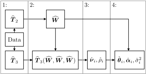
Proposition 1 suggests to retrieve the model parameters by performing matrix and tensor decompositions on the transformed moments, or rather their empirical versions. The CP decomposition (decomposition into rank-1 components as in Proposition 1) on tensors is unique under mild conditions [Kruskal, 1977]. Unfortunately, calculating the CP decomposition of a general tensor is NP hard [Hillar and Lim, 2013]. We can bypass this computational difficulty by using T2 to derive a whitening matrix that orthogonalizes the rank-1 components of T3. We describe the exact algorithm for learning the model parameters in the next section.
3 Decomposition Algorithm
Assuming linear independence of the parameter vectors θi, the matrix T2 from Proposition 1 is a real positive semidefinite symmetric matrix of rank t. Hence, there exists a rank-t decomposition T2 = U diag(γ)U ⊤ with a matrix U ∈ R(d+m)×t that has orthonormal columns and a vector γ ∈ Rt of positive eigenvalues. The whitening matrix for T2 is given by
since it holds that W ⊤T2W = I. Next, set
It can be shown that the vectors νi are orthogonal. Consequently, the tensor
has orthonormal eigenvectors νi along with scaled eigenvalues ρi = c · λ-1/2 i . Using the whitened transformed third moment T3(W,W,W), the NP-hard problem of decomposing a general tensor reduces to the decomposition of an orthogonal tensor. Decompositions of orthogonal tensors can be efficiently computed [Ge et al., 2015]. The original parameters can be retrieved by un-whitening using the pseudoinverse W † = U diag(γ 1/2 ) of W ⊤:
The practical algorithm is outlined in Algorithm 1 and also displayed as a flowchart in Figure 1. Here, we have to rely on empirical quantities, which we denote with hats. First, the transformed empirical moments ̂ T2 and ̂ T3 are derived, for which the empirical raw moments are used. Second, the rank-1 components of ̂ T3 are orthogonalized using the empirical whitening matrix ̂ W, which is obtained from ̂ T2. Third, we use the robust tensor power method from [Anandkumar et al., 2014b] to compute the t largest rank-1 components of the empirical whitened tensor ̂ T3(̂ W, ̂ W, ̂ W). In the last step, we use the un-whitening operator to obtain the final estimated model parameters. Moreover, the topic-specific variances ˆσ2 i can be calculated by solving a linear system of equations.
Importantly, Algorithm 1 runs in polynomial time: The computation of the first two steps requires O((d+m)3 ) time, the robust tensor power method is a polynomial time algorithm, and the linear system of equations can be solved and set up in polynomial time as well.
Note that the robust tensor power method finds the largest components of the whitened tensor only with high probability. Moreover, the empirical inputs of Algorithm 1 lead to errors in the estimation process. In the next section, we show that our method-of-moments estimator enjoys consistency properties nevertheless.
Algorithm 1 Method of moments for mixed topic models
Input: observed feature vectors in Rd+m
Output: model parameters (ˆ θi, ˆαi, ˆσ2 i ), i = 1, . . . , t
- 1: Compute the transformed empirical moments ̂ T2 and ̂ T3.
- 2: Compute rank-t SVD ̂ T2 = ˆU diag(ˆ γ) ˆU ⊤ and set
- 3: Compute the t largest eigenvalues ˆ ρi and corresponding eigenvectors ˆ νi of the whitened tensor ̂ T3(̂ W, ̂ W, ̂ W ).
Compute ˆσ2 i by solving a linear system of equations.
4 Consistency
In this section, we investigate when an assumed true model can be recovered from data using the proposed method-ofmoments estimator. There are two main sources of error in the estimation process. The first source are errors in the empirical moments. These errors propagate through the calculations of the transformed empirical moments as well as the whitening and un-whitening operators. The second source of error stems from performing the tensor decomposition on the empirical whitened tensor. To control the errors, we begin with a result that shows that small errors on the transformed empirical moments also imply a small error on the empirical whitened tensor.
Lemma 1. Suppose that the true matrix T2 and tensor T3 are as in Proposition 1 with linearly independent parameter vectors θi. Moreover, assume that the errors of the noisy/perturbed versions of the transformed moments satisfy
where ̂ T2 = T2 +E2 and ̂ T3 = T3 +E3. Let σmin(T2) be the smallest nonzero singular value of T2 and suppose that ε2 ≤ σmin(T2)/4. Then, it holds that
where for a universal constant C1 we define
This lemma can be proven using results from matrix perturbation theory as in [Janzamin et al., 2019]. It becomes apparent from the definition of ε that the error of the whitened tensor stems from both the estimation error of T3 (first term) and the error of the whitening procedure (second term). The next theorem, which is based on [Janzamin et al., 2019, Theorem 3.5], states that the error of the parameters (ˆ θi, ˆλi) as estimated by Algorithm 1 are small provided that the error on the whitened tensor is small.
Theorem1. In addition to the assumptions of Lemma 1, suppose that
where ρmin = mini ρi and C2 is a universal constant (the same ε as in Lemma 1 is used here). Moreover, pick any η ∈ (0, 1) and assume that the robust tensor power method performs Ω(log(t) + log log(ρmax/ε)) power updates and assume that it is restarted poly(t) log(1/η) times for each eigenvalue/eigenvector pair. Under these assumptions, Algorithm 1 estimates pairs (ˆ θ1, ˆλ1), . . . , (ˆ θt, ˆλt) in polynomial time such that with probability at least 1 - η there exists a permutation π on [t] = {1, . . . , t} for which it holds for all i ∈ [t] that
The error bounds of Theorem 1 can be understood as relative error bounds. For example, the error bound for the estimation error of ˆλi is given relative to the size of the matching eigenvalue λπ(i). Similarly, the spectral norm ‖T2‖ can be seen as an upper estimate of the scale of the parameters ˆ θi. Moreover, we point out that the error bounds become arbitrarily close to zero as ε2 → 0 and ε3 → 0 in Lemma 1 since then also ε → 0. Observe that Theorem 1 immediately implies that the errors on the Dirichlet parameters αi are also small since by Proposition 1 they differ from λi only by the constant factor α0(α0 + 1).
At this point, we briefly discuss some of the assumptions of Theorem 1 and why they are necessary. First, ε is required to be small in terms of ρmin to ensure success of the orthogonal tensor decomposition of the whitened tensor. Here, intuitively, the perturbation may not exceed the smallest component with eigenvalue ρmin of the whitened tensor because otherwise recovery becomes impossible. The required bound on ε becomes slightly stronger when more topic components need to be recovered.
The next assumptions concern the robust tensor power method. The power method iteratively generates pairs of eigenvalues and corresponding eigenvectors. The restarts guarantee that at each step the largest eigenvalue is found with high probability. The lower bound on the number of power iteration updates ensures convergence to an eigenvalue/eigenvector pair.
Based on the previous results, the next theorem shows that the method of moments is a consistent method for estimating the model parameters.
Theorem 2. Assume that Algorithm 1 is provided with data drawn from a mixed-domain topic model with parameters (θi, αi, σ2 i ), i ∈ [t] (for given α0 and number of words l). Then, Algorithm 1 yields consistent parameter estimates (ˆ θi, ˆαi, ˆσ2 i ), i = 1, . . . , t. More precisely, the estimated parameters converge in probability to the true model parameters, that is, for any δ > 0 the probabilities of the events
converge to zero as the sample size grows to infinity. □
The proof of Theorem 2 proceeds by first showing that the transformed moments ̂ T2 and ̂ T3 converge in probability to T2 and T3, respectively. In conjunction with Lemma 1 and Theorem 1, this leads to convergence in probability of ˆλi and ˆ θi. The convergence in probability of the remaining model parameters can then be easily shown. In the next section, we verify the consistency properties of our method-of-moments estimator experimentally.
5 Experiments
First, we conduct experiments on synthetic data to corroborate our theoretical findings. Then, we show on real-world data how adding images to word topic models changes the learned topics. All experiments were run on a machine with an Intel Core i9-10980XE processor with 18 cores, 128GB RAM using Python 3.8 and PyTorch 1.6.
5.1 Synthetic Data
By performing experiments on synthetic data, we want to show that the proposed method of moments can recover true model parameters effectively and efficiently. For this we define models and respectively try to recover the true known model parameters from generated samples.
Setup. In our experiments, a model configuration is defined by the number of topics t, the hyperparameter α0 = ∑ti=1 αi that controls the Dirichlet prior, the numbers of discrete and continuous features d and m, and the number l of words per document. Here, we can only sample the fivedimensional configuration space. For our experiments with synthetic data, we consider models with t ∈ {5, 10, 20} topics. Apart from that, we choose a base configuration with values α0 = 5, m = 128, d = 500, and l = 50 for the remaining parameters. Starting from this base configuration, we respectively vary one of the parameters α0, m, d, or l, while keeping the other parameters fixed.
For each configuration, we sample ten random models. Dirichlet parameters αi ∈ R+ are drawn from the uniform distribution U(0, 1) and scaled to sum up to α0. Feature mean vectors µi ∈ Rm are drawn from the uniform distribution U(-10, 10) while it is made sure that these vectors are pairwise independent. Corresponding variances σ2 i ∈ R+ are drawn from U(0, 2). For natural language topics, the frequency of any word is typically inversely proportional to its rank in the frequency table [Cohen et al., 1997], which is known as "Zipf's law". Hence, we sample word probability vectors pi ∈ Rd+ that adhere to Zipf's law.
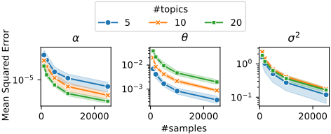
Effectiveness. We consider Algorithm 1 effective if it successfully estimates the true model parameters, where as a consequence of Theorem 2 in Section 4 we expect better recovery as the number of samples increases. For quantifying the estimation quality in our experiments, we use mean squared errors (MSEs). For the variances and parameters of the Dirichlet distribution, we use the MSEs of the vectors (σ2 i )i∈[t] and (αi)i∈[t], respectively comparing them against their estimated counterparts. For the parameter vectors θi, we use 1/t · ∑ti=1 MSE(θi, ˆ θi), where ˆ θi is the estimate of θi. We denote the different MSEs with MSEσ2 , MSEα, and MSEθ. As the estimated model parameters are permuted over the topics, we match estimated parameters and true parameters using the Kuhn-Munkres algorithm [Munkres, 1957] with matching cost MSEθ.
To confirm the consistency claims of Theorem 2, we track the MSEs for an increasing number of samples. The experimental results for the base configuration with respectively t = 5, 10, 20 topics are shown in Figure 2. All plots in Figure 2 show the mean MSEs with 95% confidence intervals computed from the respective populations of ten sampled models for each configuration. The results show that the MSEs quickly decrease towards zero as more samples are used, confirming the theoretical consistency result from Theorem 2. The same can be observed for all experimental configurations, which indicates the robustness of these results.
Efficiency. A second theoretical claim from Theorem 1 is that the method-of-moments system of equations can be solved efficiently by Algorithm 1 from Section 3. To validate this claim, we recorded the training times for different model configurations. For each configuration, we tracked the median running time of Algorithm 1 over a population of ten models. It turns out that the computation time mainly depends on the number of topics t, that is, it is almost independent from all other parameters. For instance, the running times for the base configuration and t = 10 topics are 5.1s and 6.9s for 10000 and 25000 samples, respectively. For t = 20 topics, the running times are 19.6s and 22.4s, respectively. Hence, training can be done efficiently.
5.2 Real-World Data
In order to show the real-world applicability of our model, we use a data set proposed by [Krause et al., 2017], which contains 19 511 RGB images along with single paragraphs of text describing their content. In our experiments, first, we examine the quality of the learned topics. Second, we compare the learned topics of a purely discrete (LDA) model with the topics from our mixed-domain extension. Third, we shed light on the significance of the hyperparameters t and α0. Finally, we briefly evaluate the computational performance. However, before we can learn models, some preprocessing of the data set is necessary.
Setup. For the discrete part, the text paragraphs were lemmatized and stop words as well as words that occur in less than ten documents or in more than 50% of the documents were removed. Each paragraph was then translated into a count vector over the remaining dictionary with d = 2237 words, resulting in on average 21.18 remaining words per paragraph. For the continuous part, the images were preprocessed using the first 17 layers of a pretrained ResNet18 torchvision model [He et al., 2016], yielding continuous feature vectors with m = 512 dimensions.
We tested the proposed method of moments (Algorithm 1) on the data set by learning models with t ∈ {10, 15} topics and hyperparameter values α0 ∈ {1, 50}. For each combination of α0 and t, we trained a purely discrete (LDA) topic model and our extended mixed-domain topic model.
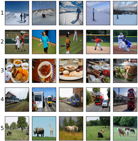
Quality of the topics. The quality of topics is still best evaluated by human inspection. Hence, we validate the discrete part by showing the words corresponding to the seven highest word probabilities for each topic. Examples are shown in Tables 1 and 2. Representing the continuous part is a little more involved. Samples from the continuous part of our model are mixtures of Gaussians: The i-th topic/mixture component has mean vector µi and mixing proportion given by the i-th entry hi of the vector h. Hence, for representing the continuous part of the topics, we solve the inference problem argmaxh p(h|y) for each image feature vector y in the data set. Then, for each topic i, we show the five images for which the inference problem yields the highest mixing proportions hi, see Figure 3.
| Topic | Most likely words (discrete topic model) |
|---|---|
| 1 | black, woman, wear, dog, person, cat, stand |
| 2 | man, wear, shirt, black, stand, blue, hold |
| 3 | table, plate, sit, pizza, food, glass, bowl |
| 4 | train, track, yellow, red, platform, blue, tree |
| 5 | giraffe, tree, grass, stand, field, zebra, elephant |
| 6 | water, boat, wave, people, sky, blue, small |
| 7 | wall, toilet, sit, cat, black, bed, room |
| 8 | plane, sky, blue, airplane, cloud, fly, red |
| 9 | building, clock, tower, large, sign, street, window |
| 10 | street, bus, sign, building, car, red, road |
The results shown in Table 1, Table 2, and Figure 3 have been obtained for t = 10 topics and α0 = 1. It can be seen that for each topic, by human judgement, the corresponding most probable words are from the same domain-both for the purely discrete and our extended mixed model. Moreover, for the mixed model, the word topics match the most representative images well.
| Topic | Most likely words (mixed topic model) |
|---|---|
| 1 | snow, ski, black, wear, man, person, tree |
| 2 | man, wear, black, tennis, shirt, baseball, blue |
| 3 | plate, table, sit, pizza, food, brown, red |
| 4 | train, bus, track, street, red, building, car |
| 5 | elephant, tree, grass, stand, brown, giraffe, zebra |
| 6 | water, blue, man, sky, wave, plane, boat |
| 7 | wall, sit, black, toilet, room, table, bed |
| 8 | plane, black, blue, sky, red, airplane, motorcycle |
| 9 | building, sign, street, tree, clock, sky, red |
| 10 | man, wear, black, people, woman, stand, elephant |
Effect of the multimodal extension. Next, we briefly discuss the differences between the purely discrete (LDA) model and our mixed-domain model extension. For our learned models, it can be observed that many topics remain similar, compare the words from Topics 2 to 8 in Tables 1 and 2. On the other hand, the visual information from the images can also lead to new topics, such as, Topic 1. The images for Topic 1 in Figure 3, which all show skiing people in snow environments, demonstrate that this new topic makes sense. Hence, adding the image modality to LDA models can lead to new insights.
Robustness. We also probed the influence of the choices for the hyperparameters t and α0 on the learned topics. Here, we can only report high-level trends due to space constraints,
Increasing t for the mixed model does not seem to remove topics: For instance, increasing the number of topics from t = 10 to t = 15, while keeping α0 = 50 fixed, did not remove any topics. The five additional topics are either completely new or result from splitting existing topics. This indicates a certain robustness of our model under the choice of t for real-world data, where the true number of topics is unknown.
The choice of the hyperparameter α0 impacts the nature of our model. If we set α0 to a small value in comparison to t, then we force most of the values of αi to be smaller than one. In this case, our model gets close to an ordinary mixture model, where each sample mostly belongs to one topic. For instance, setting α0 = 1 with t = 15 leads to unspecific topics. There are fewer unspecific topics for α0 = 50 with t = 15. In general, the mixed membership model performs better (in terms of human judgment) on our continuous deep learning features than the mixture model.
Computational aspects. Finally, we briefly touch on computational performance. As we have already observed on synthetic data, also here the running times hardly depend on α0 as well. The dependency on the number of topics t can be seen in Table 3.
| t | 2 | 5 | 10 | 15 | 20 | 25 |
|---|---|---|---|---|---|---|
| discrete | 2.66 | 3.86 | 6.53 | 9.09 | 20.24 | 27.7 |
| mixed | 7.65 | 12.49 | 22.69 | 30.92 | 47.02 | 59.47 |
6 Conclusions
We have extended the classical LDA topic model such that it also accommodates continuous features. The continuous features are modeled by mixed membership Gaussians. The parameters of the extended model can be learned in polynomial time and with statistical consistency guarantees. Such a combination of guarantees is not known for the competing maximum likelihood approach. We used synthetic data to experimentally corroborate the theoretical guarantees. Additionally, experiments on a mixed real-world data set with text and images, which we processed into continuous stateof-the-art image features, show that the mixed membership model gives qualitatively better results than a standard mixture model.
Acknowledgments
This work was supported by the German Science Foundation (DFG) grant (GI-711/5-1) within the priority program (SPP 1736) "Algorithms for Big Data", and by the Carl Zeiss Foundation within the project "A Virtual Werkstatt for Digitization in the Sciences".
@inproceedings{ijcai2021p333,
  title     = {Method of Moments for Topic Models with Mixed Discrete and Continuous Features},
  author    = {Giesen, Joachim and Kahlmeyer, Paul and Laue, Sören and Mitterreiter, Matthias and Nussbaum, Frank and Staudt, Christoph and Zarrieß, Sina},
  booktitle = {Proceedings of the Thirtieth International Joint Conference on
               Artificial Intelligence, {IJCAI-21}},
  publisher = {International Joint Conferences on Artificial Intelligence Organization},
  editor    = {Zhi-Hua Zhou},
  pages     = {2418--2424},
  year      = {2021},
  month     = {8},
  note      = {Main Track},
  doi       = {10.24963/ijcai.2021/333},
  url       = {https://doi.org/10.24963/ijcai.2021/333},
}
TY - CPAPER TI - Method of Moments for Topic Models with Mixed Discrete and Continuous Features AU - Giesen, Joachim AU - Kahlmeyer, Paul AU - Laue, Sören AU - Mitterreiter, Matthias AU - Nussbaum, Frank AU - Staudt, Christoph AU - Zarrieß, Sina T2 - Proceedings of the Thirtieth International Joint Conference on Artificial Intelligence, IJCAI-21 PB - International Joint Conferences on Artificial Intelligence Organization PY - 2021 SP - 2418 EP - 2424 DO - 10.24963/ijcai.2021/333 UR - https://doi.org/10.24963/ijcai.2021/333 ER -Copied
Machine-readable versions of this paper, for tools and AI agents:





