
Verifying Reinforcement Learning up to Infinity
Proceedings of the Thirtieth International Joint Conference on Artificial Intelligence. Main Track. Pages 2154-2160.
https://doi.org/10.24963/ijcai.2021/297
Keywords
- Machine Learning: Deep Reinforcement Learning
- Robotics: Learning in Robotics
- Multidisciplinary Topics and Applications: Validation and Verification
Abstract
Formally verifying that reinforcement learning systems act
safely is increasingly important, but existing methods
only verify over finite time.
This is of limited use for dynamical systems that run indefinitely.
We introduce the first method for verifying the time-unbounded
safety of neural networks controlling dynamical systems.
We develop a novel abstract interpretation method which,
by constructing adaptable template-based polyhedra using MILP and interval
arithmetic, yields sound---safe and invariant---overapproximations
of the reach set.
This provides stronger safety guarantees
than previous time-bounded methods and shows whether
the agent has generalised beyond the length of its training episodes.
Our method supports ReLU activation functions
and systems with linear, piecewise linear and non-linear dynamics
defined with polynomial and transcendental functions.
We demonstrate its efficacy on a range of benchmark control problems.
- [Alshiekh et al., 2018] Mohammed Alshiekh, Roderick Bloem, Rüdiger Ehlers, Bettina Könighofer, Scott Niekum, and Ufuk Topcu. Safe reinforcement learning via shielding. In AAAI, pages 2669-2678. AAAI Press, 2018.
- [Bacci and Parker, 2020] Edoardo Bacci and David Parker. Probabilistic guarantees for safe deep reinforcement learn- ing. In FORMATS, pages 231-248. Springer, 2020.
- [Bogomolov et al., 2017] Sergiy Bogomolov, Goran Frehse, Mirco Giacobbe, and Thomas A. Henzinger. Counterex- ample-guided refinement of template polyhedra. In TACAS (1), pages 589-606, 2017.
- [Brockman et al., 2016] Greg Brockman, Vicki Cheung, Lud- wig Pettersson, Jonas Schneider, John Schulman, Jie Tang, and Wojciech Zaremba. OpenAI gym. arXiv:1606.01540, 2016.
- [Bunel et al., 2018] Rudy Bunel, Ilker Turkaslan, Philip H. S. Torr, Pushmeet Kohli, and Pawan Kumar Mudigonda. A unified view of piecewise linear neural network verification. In NeurIPS, pages 4795-4804, 2018.
- [Cheng et al., 2019] Richard Cheng, Gábor Orosz, Richard M. Murray, and Joel W. Burdick. End-to- end safe reinforcement learning through barrier functions for safety-critical continuous control tasks. In AAAI, pages 3387-3395. AAAI Press, 2019.
- [Desjardins and Chaib-draa, 2011] Charles Desjardins and Brahim Chaib-draa. Cooperative adaptive cruise control: A reinforcement learning approach. IEEE Trans. Intell. Transp. Syst., 12(4):1248-1260, 2011.
- [Dutta et al., 2018] Souradeep Dutta, Susmit Jha, Sriram Sankaranarayanan, and Ashish Tiwari. Output range analy- sis for deep feedforward neural networks. In NFM, pages 121-138. Springer, 2018.
- [Ehlers, 2017] Rüdiger Ehlers. Formal verification of piece- wise linear feed-forward neural networks. In ATVA, pages 269-286. Springer, 2017.
- [Frehse et al., 2018] Goran Frehse, Mirco Giacobbe, and Thomas A. Henzinger. Space-time interpolants. In CAV (1), pages 468-486. Springer, 2018.
- [Fulton and Platzer, 2018] Nathan Fulton and André Platzer. Safe reinforcement learning via formal methods: Toward safe control through proof and learning. In AAAI, pages 6485-6492. AAAI Press, 2018.
- [Gehr et al., 2018] Timon Gehr, Matthew Mirman, Dana Drachsler-Cohen, Petar Tsankov, Swarat Chaudhuri, and Martin T. Vechev. AI2: safety and robustness certification of neural networks with abstract interpretation. In IEEE SP, pages 3-18. IEEE Computer Society, 2018.
- [Hasanbeig et al., 2019] Mohammadhosein Hasanbeig, Alessandro Abate, and Daniel Kroening. Logically- constrained neural fitted q-iteration. In AAMAS, pages 2012-2014.
- IFAAMAS, 2019.
- [Huang et al., 2017] Xiaowei Huang, Marta Kwiatkowska, Sen Wang, and Min Wu. Safety verification of deep neural networks. In CAV (1), pages 3-29. Springer, 2017.
- [Jaeger et al., 2019] Manfred Jaeger, Peter Gjøl Jensen, Kim Guldstrand Larsen, Axel Legay, Sean Sedwards, and Jakob Haahr Taankvist. Teaching stratego to play ball: Op- timal synthesis for continuous space mdps. In ATVA, pages 81-97. Springer, 2019.
- [Katz et al., 2019] Guy Katz, Derek A. Huang, Duligur Ibel- ing, Kyle Julian, Christopher Lazarus, Rachel Lim, Parth Shah, Shantanu Thakoor, Haoze Wu, Aleksandar Zeljic, David L. Dill, Mykel J. Kochenderfer, and Clark W. Barrett. The marabou framework for verification and analysis of deep neural networks. In CAV (1), pages 443-452. Springer, 2019.
- [Kendall et al., 2019] Alex Kendall, Jeffrey Hawke, David Janz, Przemyslaw Mazur, Daniele Reda, John-Mark Allen, Vinh-Dieu Lam, Alex Bewley, and Amar Shah. Learning to drive in a day. In ICRA, pages 8248-8254. IEEE, 2019.
- [Li and Bastani, 2020] Shuo Li and Osbert Bastani. Robust model predictive shielding for safe reinforcement learn- ing with stochastic dynamics. In ICRA, pages 7166-7172. IEEE, 2020.
- [Luckcuck et al., 2019] Matt Luckcuck, Marie Farrell, Louise A. Dennis, Clare Dixon, and Michael Fisher. Formal specification and verification of autonomous robotic systems: A survey. ACM Comput. Surv., 52(5):100:1-100:41, 2019.
- [Moosavi-Dezfooli et al., 2016] Seyed-Mohsen Moosavi- Dezfooli, Alhussein Fawzi, and Pascal Frossard. Deepfool: A simple and accurate method to fool deep neural networks. In CVPR, pages 2574-2582. IEEE Computer Society, 2016.
- [Sankaranarayanan et al., 2005] Sriram Sankaranarayanan, Henny B. Sipma, and Zohar Manna. Scalable analysis of linear systems using mathematical programming. In VMCAI, pages 25-41. Springer, 2005.
- [Schulman et al., 2017] John Schulman, Filip Wolski, Pra- fulla Dhariwal, Alec Radford, and Oleg Klimov. Proximal policy optimization algorithms. arXiv:1707.06347, 2017.
- [Singh et al., 2019] Gagandeep Singh, Timon Gehr, Markus Püschel, and Martin T. Vechev. An abstract domain for certifying neural networks. Proc. ACM Program. Lang., 3(POPL):41:1-41:30, 2019.
- [Tjeng et al., 2019] Vincent Tjeng, Kai Y. Xiao, and Russ Tedrake. Evaluating robustness of neural networks with mixed integer programming. In ICLR (Poster). OpenRe- view.net, 2019.
- [Tran et al., 2020] Hoang-Dung Tran, Xiaodong Yang, Die- go Manzanas Lopez, Patrick Musau, Luan Viet Nguyen, Weiming Xiang, Stanley Bak, and Taylor T. Johnson. NNV: the neural network verification tool for deep neural net- works and learning-enabled cyber-physical systems. In CAV (1), pages 3-17. Springer, 2020.
- [Xiang et al., 2018] Weiming Xiang, Hoang-Dung Tran, and Taylor T. Johnson. Output reachable set estimation and verification for multilayer neural networks. IEEE Trans. Neural Networks Learn. Syst., 29(11):5777-5783, 2018.
References were extracted automatically from the PDF and may contain errors.
Full text extracted automatically from the PDF; figures, tables and equations may differ. The PDF is the version of record.
1 Introduction
Reinforcement learning (RL) has reached super-human capabilities on many challenging problems and is being increasingly applied to cyber-physical tasks, such as robot control and autonomous driving [Kendall et al., 2019]. The criterion for training and evaluating RL agents is traditionally their performance, that is, how quickly and efficiently they solve their task. However, for agents that interact with critical environments, performance must meet safety: not only is it required that positive outcomes eventually happen, but also that negative ones do not [Fulton and Platzer, 2018; Luckcuck et al., 2019]. Safety is subtle, because a system is truly safe only if it avoids danger regardless of how long it is left running. Determining whether an RL system is safe for unbounded time addresses both a formal verification question, providing stronger guarantees of correctness than bounded verification, and a machine learning question, indicating whether the learning algorithm has generalised a strategy beyond the length of the episodes used to train it. Verifying RL requires reasoning about the dynamics of the environments together with the learned agents which, in modern RL, are neural networks. For the first time, we treat the automated (and sound)
time-unbounded verification of neural networks interacting with dynamical systems.
Safety analysis for neural networks has been studied before for bounded settings. One example is classification, whose well-known vulnerability to adversarial attacks has been analysed using gradient descent, mixed-integer linear programming (MILP), and satisfiability modulo theories (SMT) [Moosavi-Dezfooli et al., 2016; Huang et al., 2017; Ehlers, 2017; Bunel et al., 2018; Katz et al., 2019]. Searchbased algorithms of this kind are inherently bounded, unlike abstract interpretation methods. Abstract interpretation computes a representation of the set of reachable states and checks whether it avoids a set of bad states. Methods for the abstract interpretation of neural networks have borrowed from the analysis of numerical programs, and have been applied to adversarial attacks [Gehr et al., 2018; Singh et al., 2019], output range analysis [Xiang et al., 2018; Dutta et al., 2018], and time-bounded verification of RL [Tran et al., 2020; Bacci and Parker, 2020]. Time-unbounded verification is more difficult because it requires that the abstraction is both safe, i.e., disjoint from the bad states, and invariant, i.e., no other states are reachable from it; none of the available approaches, as is, have been demonstrated to achieve both requirements on RL problems.
We present the first technique for verifying whether a neural network controlling a dynamical system maintains the system within a safe region for unbounded time. For this purpose, we overapproximate the reach set using template polyhedra, i.e., polyhedra whose shape is determined by a set of directions, the template [Sankaranarayanan et al., 2005]. Traditional interval and octagonal abstractions have rigid shapes which often produce abstractions that are too coarse to be safe or too tight to be invariant. By contrast-with an appropriate choice of directions-template polyhedra can be adapted to the verification problem making the abstraction tight only where necessary and thus facilitating the identification of safe invariants [Bogomolov et al., 2017; Frehse et al., 2018].
We formulate the problem of computing template polyhedra as an optimization problem. For this purpose, we introduce an MILP encoding for a sound abstraction of neural networks with ReLU activation functions acting over discrete-time systems. We support linear, piecewise linear and non-linear systems defined with polynomial and transcendental functions. For the latter, we combine MILP with interval arithmetic.
We propose a safety verification workflow where agents trained with any, possibly model-free, RL technique are verified against a model of the environment. Every model is accompanied with user-defined templates which, as we experimentally demonstrate, suffice to verify multiple agents. Upon every successful verification result we thus certify that an agent is safe w.r.t. a model, which determines our safety specification. Ultimately, we provide formal guarantees that are equivalent to (or stronger than) those of agents that are trained or enforced to be safe [Alshiekh et al., 2018; Cheng et al., 2019; Hasanbeig et al., 2019; Li and Bastani, 2020],yet without imposing constraints on the agent or the RL process.
We demonstrate that our method effectively verifies agents trained over three benchmark control problems [Jaeger et al., 2019; Tran et al., 2020; Brockman et al., 2016]. We additionally show that an alternative time-unbounded verification approach built upon range analysis fails in all cases.
In summary, we introduce the first method for the formal time-unbounded safety analysis of RL systems. We have built a software prototype and demonstrate the efficacy of our method over a range of benchmarks.
2 Safety Analysis of Reinforcement Learning
A time-invariant controlled dynamical system with discrete actions and over discrete time consists of an n-dimensional vector of real-valued state variables x, an m-dimensional vector of real-valued observable variables y, and a natural number Σ of input actions available to an external agent. The set A denotes the set of actions {a ∈ Z: 1 ≤ a ≤ Σ}. The system dynamics are determined by a difference equation
where xt ∈ Rn , at ∈ A, and ct respectively denote state, input action, and control disturbance at time t. The set C ⊂ Rn is the space of control disturbances, X0 ⊂ Rn is the space of initial conditions, and f : Rn × A → Rn is the update function. An observation function g : Rn → Rm and a space of observation disturbances D ⊂ Rm determine the observable values at time t from a state:
A trajectory of the system is an infinite sequence of states and actions in alternation
where every state x1, x2, . . . is determined by Eq. (1); every action a1, a2, . . . is determined by an external agent σ : Rm → A from the observation at the previous step, i.e.,
We target the safety verification question for controlled dynamical systems. Let B ⊂ Rn be a set of bad states. Verifying the safety of a system consists of deciding whether, for every trajectory x0a1x1a2x2 . . . , we have that xt ̸∈ B for all t = 0, . . . ,∞. Dually, it consists of determinining whether there exists a finite prefix x0a1x1 . . . akxk such that xk ∈ B. In the former case we say that the system is safe; in the latter we say that it is unsafe.
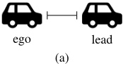
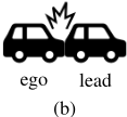
Example 1. Adaptive cruise control is a paradigmatic example for the safety of an RL system [Desjardins and Chaib-draa, 2011; Tran et al., 2020]. In its simplest form, it consists of two vehicles, ego and lead, moving in a straight line. An agent should control ego so that it stays at some close and safe distance from lead. State variables xv, x′v , and x′′ v resp. determine position, speed, and acceleration of each vehicle v = ego, lead. The observation function exposes vehicles distance xlead - xego and speed of ego x′ego ; both observables are subject to a disturbance. Lead proceeds at a constant speed of 28ms-1 and, at every step, the agent can either decelerate (action 1) or accelerate ego by 1m s-2 (action 2). Update and observation functions are shown in Sect. 4.2. The agent is safe only if the distance is positive along every trajectory (Fig. 1a); every other condition indicates that the vehicles have crashed (Fig. 1b). The set of bad states is thus defined by the constraint xlead ≤ xego. Trivially, an agent that always decelerates is safe; however, safety must coexist with performance, which rewards the agent for keeping ego close to lead.
For the purpose of training an agent using RL, we augment the system with the probability distributions λX0 , λC, and λD for the sets X0, C, and D, respectively. We require that supp(λX0 ) = X0, supp(λC) = C, and supp(λD) = D, where supp(λ) = {x: λ(x) > 0} is the support of distribution λ. This induces a discrete-time partially observable Markov decision process (POMDP) with finite actions and possibly uncountable state space and branching. Precisely, we let Rn be the state space and Rm be the observation space, together with the σ-algebras FX and FY of measurable subsets of respectively Rn and Rm. The probability of beginning from a set X is given by the initial belief µ: FX → [0, 1], i.e.,
The set of actions A corresponds to that of the original controlled dynamical system. The transition probability function T : Rn ×A×FX → [0, 1] is thus
which denotes the probability that, from state x and after choosing action a, the process jumps to a target set Z. The observation probability function O: Rn × FY → [0, 1] is
that is, the probability of observing subset Y from state x. Finally, a reward function R: Rm → R maps observations to reward values. We discuss in Sect. 4 how we design rewards functions for obtaining performant and safe agents using RL.
Agents are given in the form of neural networks. We consider neural networks with ReLU activation functions, m input neurons, l hidden layers with respectively h1, . . . , hl neurons, and Σ output neurons. The variable vectors z0, . . . , zl+1 denote the values of the neurons at each layer. The input layer z0 is assigned from the system observation y, every hidden layer is determined according to the equation
and the output layer according to zl+1 = Wl+1zl. Each matrix Wi denotes the weights between any other (i - 1)-th and i-th layers, and each vector bi denotes the respective biases. The function ReLU applies max{·, 0} element-wise to its hi-dimensional argument. The output action is determined by the index of the output neuron whose value is the highest; in other words, the neural network defines the agent
where ej is the j-th standard unit vector of RΣ and 〈·, ·〉 denotes scalar product. Altogether, the neural network acts as a classifier from observations to actions.
We train our agents over the POMDP induced by the distributions over initial and disturbance sets. Then, we verify the safety of the dynamical system controlled by the obtained network. We tackle time-unbounded safety verification; for this purpose, we introduce a technique for constructing coarse yet safe abstractions of the reach sets of these neurally controlled dynamical systems.
3 Template-based Polyhedral Abstractions for Neurally Controlled Dynamical Systems
We employ abstract interpretation for constructing a sound overapproximation of the reach set of the system. Specifically, we compute a sequence of abstract sets of states in Rn
for increasing t ≥ 0, where post-the post operator-ensures that Xt+1 overapproximates the states that are reachable after one step from Xt. Time-unbounded safety verification succeeds if our procedure finds a finite k ≥ 1 such that the sequence up to k is
The procedure computes Xt iteratively for increasing t and checks both conditions at each step. If both are satisfied the procedure terminates concluding that the system is safe; if safety is violated it terminates with an inconclusive answer. This procedure may, in the worst case, not terminate. We present a post operator that computes Xt in the form of finite unions of template polyhedra; as our experiments show (Sect. 4), this yields safe and invariant abstractions in practice.
We call a finite set of directions ∆ ⊂ Rn a template. A ∆-polyhedron is a polyhedron whose facets are normal to the directions in ∆. The ∆-polyhedron of X, where X is a convex set in Rn , is the tightest ∆-polyhedron enclosing X:
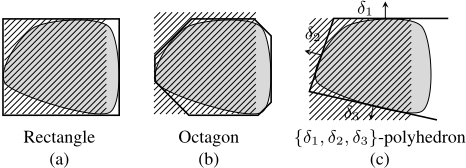
where ρX(δ) = sup{〈δ, x〉 : x ∈ X} is the support function of X. Special cases of template polyhedra are rectangles (i.e., intervals) and octagons (Fig. 2a and b), which are determined by specific templates. In addition, by using fewer, well-chosen directions, template polyhedra let us construct sufficiently tight yet unbounded polyhedral abstractions (Fig. 2c).
We compute template polyhedra over a symbolic representation of the post. We split the post computation into a partitioning Pt (a set of sets in Rn ) that overapproximates the state that are reachable after one step fromXt, i.e.,
As we show below, we build the partitioning from the piecewise structure of the system and represent its elements symbolically. Then, for every symbolic representation we construct a template polyhedron by optimising in the directions of ∆. Our post is the union of these template polyhedra:
where convP ′ denotes the convex hull of the members of P ′ ⊂ Rn . The post produces a union of convex polyhedral overapproximations.
Neurally controlled dynamical systems often have piecewise dynamics. The discrete action space naturally induces a case split in the update function. Also, some systems may have dynamics that switch between two or more behaviours according to guard conditions over the state (see, e.g., Sect. 4.1). Formally, each case split is a partial function from a set F ⊂ (Rn × A → Rn ) s.t. f = ∪F and f is total. Likewise, this case split and the encoding below also applies to the observation function g; for simplicity, we only refer to f.
We compute post(Xt) using optimisation. We express an encoding for every combination of action a ∈ A, case split f ′ ∈ F of the update function, and convex polyhedron X′ from the finite union of convex polyhedra Xt; each combination induces an element P ′ of Pt. For a direction δ ∈ ∆, we solve the following problem:
over the variables c, x′ , p′ ∈ Rn and y, d ∈ Rm. The solution provides the value of ρconvP ′(δ) which, computed over all δ ∈ ∆, yields the ∆-polyhedron of P ′ (see Eq. (11)); in turn, the polyhedron yields an element of the post (see Eq. (13)).
The optimisation problem consists of a linear objective function and constraints for, respectively, the action chosen by the neural network, update and observation functions, and disturbance and input sets. We assume that the disturbance sets C and D are convex polyhedra, and that the initial set X0 is a union of convex polyhedra similarly to all other Xt for t ≥ 1. For partial functions f ′ (·, a), we assume that the domains of definition are given as convex polyhedra. Consequently, the constraints for C, D, X′ , and dom(f ′ (·, a)) are expressed with systems of linear inequalities. Our encoding for the constraint over the neural network σ(y) = a and our overapproximation of non-linear functions introduce integer variables, as we show below. The optimisation problem thus results in an MILP.
The network selects action a when the value of the a-th output neuron is larger than the value of all other output neurons (Eq. (9)). The constraint for σ(y) = a is thus
where zl+1 ∈ RΣ is a variable for the value of the output layer. For each hidden layer i, we add to the optimisation problem a real variable zi ∈ Rhi for the values of the neurons in the layer, plus an integer variable z′i ∈ Zhi for the activation status of the ReLU function. We encode the ReLU function using a big-M encoding [Tjeng et al., 2019]. For the hidden layers, we add constraints
For output and input layers, we add zl+1 = Wl+1zl and z0 = y. Constant M ∈ R is an upper bound for the values a neuron can take, which we set to a sufficiently large value so as not to constrain the system's states.
Linear update (and observation) functions are encoded directly into the MILP using linear equalities. For non-linear constraints defined with polynomials or transcendental functions, we introduce an overapproximation based on interval arithmetic. Constraint p′ = f ′ (x′ , a) + c is an n-dimensional system of equalities. We identify the equations within the the system that are non-linear and let p′N , f ′N , and cN be the corresponding projection for resp. p′ , and f ′ , and c. Moreover, we let x′N be the largest subset of variables in x′ that appear in these non-linear equations. The non-linear components thus form the reduced system
We encode the remaining linear components exactly, using linear equalities, whereas we overapproximate Eq. (17). First, we construct a bounding box of X′N ; note that we ensure beforehand that X′N is bounded with an appropriate template choice (see Sect. 4.3). Then, we partition the bounding box into a grid of intervals [ξ 1 , ¯ ξ1], . . . , [ξκ , ¯ ξκ]. For every element i = 1, . . . , κ, we compute using interval arithmetic an output interval [πi, ¯πi] for the image of [ξ i , ¯ ξi] though f ′N(·, a). As a result, we obtain a lookup table that associates input intervals to output intervals. We encode this table by adding to the MILP the integer variables ζ1, . . . ζκ ∈ Z, each of which represents an active interval, and the following constraints:
We tune the precision of the overapproximation by fixing a desired granularity for output intervals, a maximal diameter, and iteratively split the input intervals until that is attained.
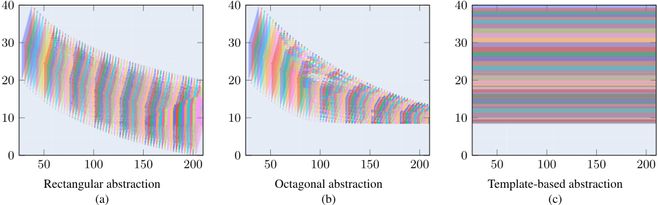
Example 2. We trained a neural network for adaptive cruise control (Ex. 1) by rewarding the agent for keeping a safety distance of 10m; the vehicles start from a range of distances between 20 and 40m. We employed our method for analysing its safety using three different abstraction templates: rectangles, octagons and a custom template designed for this system (see Sect. 4.2). Rectangles produce an excessively coarse abstraction which hit distance zero: the bad state (Fig. 3a). Unlike rectangles, octagons keep track of the vehicles' distance and thus avoid the bad state; however, their abstraction is too tight to identify an invariant, inducing an infinite sequence of polyhedra along the vehicles' position (Fig. 3b). Our custom template keeps track of vehicles' distance, while abstracting away absolute position; this yields a safe and invariant abstraction of the reach set (Fig. 3c).
4 Experimental Evaluation
We evaluate our method over multiple agents for 3 benchmark control problems: a bouncing ball, automated cruise control, and cart-pole. We selected a range of loss functions and hyperparameters and verified, using our method, which setups produce safe behaviour. We trained RL agents using proximal policy optimisation (PPO) [Schulman et al., 2017]. We used standard feed forward architectures with 2 hidden layers of size 64 (32 for the bouncing ball), and ReLU activation functions; we used a learning rate of 5e-4 .
We built a prototype 1 and verified the safety of these networks with rectangular and octagonal abstractions and, when necessary, custom templates 2 which we discuss in Sect. 4.2 and 4.3. In addition, we also compared our method with an alternative approach built upon range analysis (Sect. 4.4).
We ran our experiments on a 4-core 4.2GHz with 64GB RAM. Results are shown in Tab. 1 and discussed in Sect. 4.4.
4.1 Bouncing Ball
Environment. The system consists of a ball, whose height from the ground is determined by a variable x and whose vertical velocity is determined by a variable x′ [Jaeger et al., 2019]. Under normal conditions, position is given by the equation xt = xt-1 + τ · x′t-1 and velocity is given by x′t = x′t-1 - τ · g, where g denotes gravitational acceleration and τ = 0.1 indicates our time step. Every time the ball hits the ground, i.e., xt-1 ≤ 0, the ball bounces back after losing 10% of its energy, i.e., x′t = -0.9 · x′t-1 - τ · g and xt = 0. At every timestep, the agent can either hit the ball downward by adding -4ms-1 to its velocity, or do nothing. Overall, this results in a piecewise linear system.
Training. The goal is to ensure that the ball keeps bouncing indefinitely, while using the piston as little as possible. We reward the agent with value 1 for each time step that the ball's absolute velocity is above the minimal velocity of 1ms-1 . Additionally, we discourage the agent from overactivating the piston by punishing it with reward -1 every time it is activated. We trained 11 agents using different initial seeds and with episodes of at most 1000 steps, after which we forcefully terminate. We terminate training either when our agent reaches a mean reward of 900 or after 5M training steps.
Verification. As initial condition, we consider the set of initial ball heights x0 ∈ [7, 10] and initial velocities x′0 ∈ [0, 0.1]. We use traditional rectangular and octagonal abstractions, that is, for rectangles we use the directions x,-x, x′ ,-x′ and for octagons add the extra directions x+x′ , -x+x′ , x-x′ , -xx′ . Notably, all agents have been successfully verified with both rectangles and octagons with no notable difference in performance.
4.2 Adaptive Cruise Control
Environment. The problem consists of two vehicles, lead and ego, whose state is determined by variables xv, x′v and x′′ v , respectively, for position, speed, and acceleration of v = ego, lead (see Ex. 1). The lead car proceeds at constant speed
1 https://github.com/phate09/SafeRL Infinity
2 For readability, we present direction δ by displaying 〈δ, x〉.
(28 m s-1 ), and the agent controls the acceleration (± 1 m s-2 ) of ego using either of two actions. Its dynamics are given by
The observation function exposes vehicle distance ydis and the velocity of ego yvel with an additional observation disturbance of radius ϵ, determined by the following equations:
We consider a case with ϵ = 0 and another case with ϵ = 0.05, and use τ = 0.1. Altogether, when an action is given this is a linear system with disturbances.
Training. We train our agents using two 2 different reward functions. A "simple" function only rewards the agent for each timestep it survives without crashing, that is, R(ydis, yvel) = 1; a "complex" function additionally punishes the agent from being away from a predefined distance y⋆ dis , specifically, R(ydis, yvel) = 1-0.02 · (ydis -y⋆ dis )2 . We cap each episode at 1000 timesteps. From the definition of the simple cost function above, we can periodically pre-test the safety of the agent by disabling the exploration and requiring an average score of 1000 before attempting the verification step. For the complex cost function it is more difficult to estimate what a safe score should be, so we empirically determined that before attempting to verify the neural network, the agent needs to reach an average score of at least -20. As an additional stopping condition we terminate the training after 20M training steps. We ran our algorithm over 22 agents trained with different initialisation seeds and two modes of input perturbation (ϵ = 0 and ϵ = 0.05) for up to 300 seconds.
Verification. We consider the initial region enclosed within the constraints xlead,0 ∈ [40, 50], xego,0 ∈ [0, 10], x′ego,0 = 36. Using standard rectangular or octagonal abstractions that verification procedure fails by either returning a spurious counterexamples or timing out. To effectively verify this systems, we designed a template with the following directions: x′′ ego , -x′′ ego , x′lead , -x′lead , (x′lead -x′ego ), -(x′lead -x′ego ), (xlead -xego), -(xlead -xego). This allows us to keep track of the distance between the two vehicles and easily spot if the agent encounters an unsafe state, while enabling the identification of an invariant. Agents could be proven to be safe in most but not all of the cases within our time constraints (300s), showing a higher degree of difficulty compared to the previous problem. When testing the agents on the perturbed environment, only a few of the agents that were proven safe in the previous experiment retained safety, demonstrating that the problem the agent had to solve is much harder.
4.3 Cart-pole
Environment. The cart-pole problem is a very well known control problem in the RL literature; for our experiments, we refer to the OpenAI Gym implementation of CartPolev1 [Brockman et al., 2016]. The state variables are angle θ
and angular velocity θ′ of the pole, together with horizontal position x and velocity x′ of the cart. The agent has two actions for pushing the cart to either the left or the right which, together with θ and θ′ , internally determine horizontal and angular accelerations x′′ and θ′′ . The values of θ′′ and x′′ are determined according to non-linear equations defined with transcendental functions and whose arguments are the action and variables θ and θ′ . The update rule for angle θ, position x, and velocities θ′ and x′ follow a linear Euler integration rule with timestep τ . All variables x, x′ , θ, and θ′ are observable.
Training. The objective for an agent is to keep the pole upright; we consider the system unsafe whenever θ > 12◦ , according to the OpenAI Gym termination condition. We train agents using three cost functions. A "simple" version only rewards the agent for surviving; a "complex" version discourages it from having high values of θ and θ′ , i.e., R(x, x′ , θ, θ′ ) = 1 - 0.5 ∗ θ2 - 0.5 ∗ (θ′ )2 - 0.1 ∗ (x′ )2 ; a third one limits the complex cost function to only giving positive rewards. For every cost function, we trained two agents using τ = 0.02 and τ = 0.001, thus obtaining 6 agents. We capped each episode to 8000 timesteps. For all cost functions, we terminate training when the mean reward of the last 50 episodes reaches 7950 (i.e., sufficiently close to the maximum of 8000) or after 20M training steps. We use curriculum learning to improve training: when the mean episode return reaches 6500 the initial states get sampled from bigger intervals with θ ∈ [-0.2, 0.2] and θ′ ∈ [-0.5, 0.5].
Verification. We use the starting region of OpenAI Gym, i.e., all variables are initialised from the interval [-0.05, 0.05]. However, we remove the constraints imposed on x and let the cart-pole move freely to any position. Rectangles and octagons failed to prove safety on all instances. Thus, we designed a custom template that forms an octagon over θ and θ′ only, determined by the following directions: θ, -θ, θ′ , -θ′ , θ + θ′ , -θ + θ′ , θ - θ′ , -θ - θ′ . This template choice serves two purposes. First, it ignores position x thus abstracting its values away. Second, it bounds the space of θ and θ′ , which are the variables appearing in the non-linear equations of the system. This lets us use interval arithmetic for encoding the non-linear equations in our MILP (see Sect. 3). We verified our agents against both versions of the environment, with τ = 0.02 and with τ = 0.001 to test the how it would affect safety. The agents that did run on environments at τ = 0.001 during the evaluation found an invariant quicker and in less timesteps.
4.4 Results
Table 1 reports number of solved instances, average timestep of invariant detection, number of template polyhedra in the abstract reach set after pruning redundant ones, and runtime.
The time required to find whether the agent is safe increases as the number of variables in the problem increases (BB has 2, ACC has 6 and CP has 4) and on the type of abstraction. Templates enable us to find invariants on problems that would not converge otherwise (ACC and CP). Once we introduce a small observation perturbation on ACC such as in adversarial examples, only a small fraction of the agents remain safe negatively impacting safety.
From our results, the cost function used does not strongly correlate with the safety of the agent hence it is omitted in the table. Conversely, shorter timesteps contribute positively to reducing the time required to verify an agent, promoting a higher chance to find a safe invariant in early timesteps.
| Env. | Abs. | Safe | Avg k | Avg poly. | Avg runtime |
|---|---|---|---|---|---|
| BB | Rect | 11/11 | 237 | 477 | 40s |
| BB | Oct | 11/11 | 203 | 411 | 47s |
| ACC (ϵ = 0) | Temp | 20/22 | 467 | 610 | 171s |
| ACC (ϵ = .05) | Temp | 5/22 | 226 | 337 | 124s |
| CP (τ = .001) | Temp | 4/6 | 27 | 18 | 67s |
| CP (τ = .02) | Temp | 3/6 | 100 | 125 | 174s |
Additionally, we verified our agents using a naive timeunbounded approach (based on range analysis) that constructs, from the network in isolation, ranges of observables for which an action is enabled; then, it uses these ranges as guards for the dynamical system. This alternative approach failed on all instances by producing inconclusive answers (unsafe abstractions) or reaching time-out. Notably, existing verification methods for neural networks are incomparable as they only support time-bounded problems such as robustness to adversarial attacks or finite-horizon safety analysis of RL [Tran et al., 2020; Gehr et al., 2018].
5 Conclusion
We presented the first method for verifying the safety of RL agents up to infinite time. To this end, our method constructs coarse, yet precise enough, abstractions using template polyhedra. We demonstrated the efficacy of our method over multiple case studies. Our technique yields stronger formal guarantees than previous time-bounded methods, and also indicates which RL setups generalise well beyond the length of their training episodes. Our result poses the basis for future research, both in machine learning and formal verification. Our method can be used to make informed decisions about architectures and hyperparameters, and also to guide an RL procedure that trains for safety. Also, our method lends itself to extensions towards multi-agent systems, systems over continuous time, continuous actions and automated abstraction refinement.
Acknowledgments
We thank Hosein Hasanbeig and the anonymous reviewers for their suggestions. This work was in part supported by the HICLASS project (113213), a partnership between Aerospace Technology Institute (ATI), Department for Business, Energy & Industrial Strategy (BEIS) and Innovate UK, and the European Research Council (ERC) under the European Union's Horizon 2020 research and innovation programme (grant agreement No. 834115, FUN2MODEL).
@inproceedings{ijcai2021p297,
  title     = {Verifying Reinforcement Learning up to Infinity},
  author    = {Bacci, Edoardo and Giacobbe, Mirco and Parker, David},
  booktitle = {Proceedings of the Thirtieth International Joint Conference on
               Artificial Intelligence, {IJCAI-21}},
  publisher = {International Joint Conferences on Artificial Intelligence Organization},
  editor    = {Prof. Zhi-Hua Zhou},
  pages     = {2154--2160},
  year      = {2021},
  month     = {8},
  note      = {Main Track},
  doi       = {10.24963/ijcai.2021/297},
  url       = {https://doi.org/10.24963/ijcai.2021/297},
}
TY - CPAPER TI - Verifying Reinforcement Learning up to Infinity AU - Bacci, Edoardo AU - Giacobbe, Mirco AU - Parker, David T2 - Proceedings of the Thirtieth International Joint Conference on Artificial Intelligence, IJCAI-21 PB - International Joint Conferences on Artificial Intelligence Organization PY - 2021 SP - 2154 EP - 2160 DO - 10.24963/ijcai.2021/297 UR - https://doi.org/10.24963/ijcai.2021/297 ER -Copied
Machine-readable versions of this paper, for tools and AI agents:





