Finite-Trace and Generalized-Reactivity Specifications in Temporal Synthesis

1 Introduction

Program synthesis is considered the culmination of the ideal of declarative programming [Finkbeiner, 2016; Ehlers et al., 2017]. By describing a system in terms of what it should do, instead of how it should do it, we are able, on the one hand, to simplify the program design process while avoiding human mistakes and, on the other hand, to allow an autonomous agent to self-program itself just from high-level specifications. Linear Temporal Logic (LTL) synthesis [Pnueli and Rosner, 1989] is possibly one of the most popular variants of program synthesis, being the problem of automatically designing a reactive system with the guarantee that all its behaviors comply with desired dynamic properties expressed in LTL, the most used system/process specification language in Formal Methods. Unfortunately this dream of LTL synthesis has proven to be too difficult, and, in spite of a full-fledged theory, we still do not have good scalable algorithms after more than 30 years [Kupferman, 2012].

∗Corresponding Author

There have been two successful responses to these difficulties, both having to do with limiting the expressive power of the formalism used for the specification. The first approach, developed in Formal Methods, has been what we may call the GR(1), response [Bloem et al., 2012]: essentially you focus on safety conditions, determining the possible transitions in a game between the environment and the agent, plus one powerful notion of fairness called Generalized Reactivity(1), or GR(1). This approach has found numerous applications, for example, in robotic motion-and-mission planning [KressGazit et al., 2009]. The second approach, developed in AI and inspired by classical AI planning, is of finite-horizon temporal synthesis, with LTLf (LTL on finite traces) [De Giacomo and Vardi, 2013] as the specification language. In this approach [De Giacomo and Vardi, 2015], we specify the agent's goal in LTLf , together possibly with some assumptions on the environment, such as safety conditions, possibly specified as a nondeterministic planning domains [Camacho et al., 2017; De Giacomo and Rubin, 2018; Aminof et al., 2018; Camacho et al., 2018; He et al., 2019], or simple fairness and stability conditions (both special cases of GR(1) fairness) [Zhu et al., 2020]. There are also studies in which general LTL assumptions are used for LTLf goals, but in this case the difficulties of handling LTL can indeed manifest [Camacho et al., 2018; Aminof et al., 2019; De Giacomo et al., 2020b]. Since LTLf is a fragment of LTL, as shown in [De Giacomo and Vardi, 2013], the problem of LTLf synthesis under LTL assumptions can be reduced to LTL synthesis, as, e.g., explicitly pointed out by [Camacho et al., 2018]. However, LTL synthesis algorithms do not scale well due to the difficulty of B¨uchi automata determinization, see e.g., [Finkbeiner, 2016].

In this work we propose to take these two lines of work, which are really the only successful stories in LTL synthesis, and bring them together. We first study the case in which we have an LTLf agent goal and a GR(1) assumption. We propose an approach based on using the automaton corresponding to the LTLf goal as the game arena on which the environment has to satisfy its GR(1) assumption. This means that we are able to reduce the problem to that of GR(1) synthesis over the new arena. We prove the correctness of the approach.

We then add to the framework safety conditions for both the environment and the agent, obtaining a highly expressive yet still scalable form of LTL synthesis. These two kinds of safety conditions differ, since the environment needs to maintain its safety indefinitely (as usual for safety), while the agent has to maintain its safety conditions only until s/he fulfils its LTLf goal, i.e., within a finite horizon, something that makes them similar to "maintenance goals" in Planning [Ghallab et al., 2004]. We show that we can specify these safety conditions in a very general way by using LTLf . In particular, our safety conditions require that all prefixes of a trace satisfy an LTLf formula. For the environment safety conditions we consider all finite prefixes of infinite traces, while for the agent safety conditions we consider all prefixes of the finite trace satisfying the agent's LTLf goal. Again we prove the correctness of our approach and demonstrate its scalability through an experimental analysis.

2 Preliminaries

LTL and LTLf . LTL is one of the most popular logics for temporal properties [Pnueli, 1977]. Given a set of propositions Prop, the formulas of LTL are generated as follows:

• π, i |= a iff a ∈ πi (for a ∈ Prop);

where a ∈ Prop. We use common abbreviations, so we have eventually as ✸ϕ ≡ true U ϕ and always as ✷ϕ ≡ ¬✸¬ϕ. LTL formulas are interpreted over infinite traces π ∈ (2Prop )ω . A trace π = π0, π1, . . . is a sequence of propositional interpretations (sets), where for every i ≥ 0, πi ∈ 2Prop is the i-th interpretation of π. Intuitively, πi is interpreted as the set of propositions that are true at instant i. Given π, we define when an LTL formula ϕ holds at position i, written as π, i |= ϕ, inductively on the structure of ϕ, as:

• π, i |= ¬ϕ iff π, i ̸|= ϕ;
• π, i |= ©ϕ iff π, i +1 |= ϕ;
• π, i |= ϕ1 ∧ϕ2 iff π, i |= ϕ1 and π, i |= ϕ2;
• π, i |= ϕ1 U ϕ2 iff there exists j ≥ i such that π, j |= ϕ2, and for all k, i ≤ k < j we have that π, k |= ϕ1.

LTLf is a variant of LTL interpreted over finite traces instead of infinite traces [De Giacomo and Vardi, 2013]. The syntax of LTLf is exactly the same to the syntax of LTL. We define π, i |= ϕ, stating that ϕ holds at position i, as for LTL, except that for the temporal operators we have:

We say π satisfies ϕ, written as π |= ϕ, if π, 0 |= ϕ.

• π, i |= ©ϕ iff i < last(π) and π, i + 1 |= ϕ;

where we denote the last position (i.e., index) in the finite trace π by last(π). In addition we define the weak next operator · as abbreviation of ·ϕ ≡ ¬©¬ϕ. Note that, over finite traces, ¬©ϕ ̸≡ ©¬ϕ, instead ¬©ϕ ≡ ·¬ϕ. We say that a trace satisfies an LTLf formula ϕ, written π |= ϕ, if π, 0 |= ϕ.

• π, i |= ϕ1 U ϕ2 iff there exists j such that i ≤ j ≤ last(π) and π, j |= ϕ2, and for all k, i ≤ k < j we have that π, k |= ϕ1.

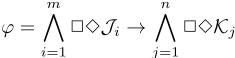
Generalized Reactivity(1) formulas. Generalized Reactivity(1) [Piterman et al., 2006], or GR(1), is a fragment of LTL that generalizes fairness (✷✸ϕ) and stability (✸✷ϕ) formulas (cf. [Zhu et al., 2020]). Given a set of propositions Prop, a GR(1) formula ϕ is required to be of the form where Ji and Kj are Boolean formulas over Prop.

Deterministic Automata. A deterministic automaton (DA, for short) is a tuple A = (Σ, S, s0, δ, α), where Σ is a finite alphabet, S is a finite set of states, s0 ∈ S is the initial state, δ : S × Σ → S is the transition function, α ⊆ Sω is an acceptance condition. Given an infinite word w = a0a1a2 . . . ∈ Σω , the run of A on w, denoted by A(w) is the sequence r = s0s1s2 . . . ∈ Sω starting at the initial state s0 where si+1 = δ(si, ai). The automaton A accepts the word w if A(π) ∈ α. The language of A, denoted by L(A), is the set of words accepted by A. In this work we specifically consider reachability, safety, and reachability-safety acceptance conditions:

Reachability conditions. Given a set T ⊆ S of target states, Reach(T) = {s0s1s2 . . . ∈ Sω | ∃k ≥ 0 : sk ∈ T} requires that a state in T is visited at least once.

Safety conditions. Given a set T ⊆ S of target states, Safe(T) = {s0s1s2 . . . ∈ Sω | ∀k ≥ 0 : sk ∈ T} requires that only states in T are visited. This is the dual of reachability conditions.

Reachability-Safety conditions. Given two sets T1, T2 ⊆ S of target states corresponding to reachability and safety conditions, respectively, Reach - Safe(T1, T2) = {s0s1s2 . . . ∈ Sω | ∃i ≥ 0 : si ∈ T1 and ∀j, i ≥ j ≥ 0 : sj ∈ T2} requires that a state in T1 is visited at least once, and until then only states in T2 are visited.

We define the complement of a DA A = (Σ, S, s0, δ, α) as A = (Σ, S, s0, δ, Sω \α). Note that L(A) = Σω \L(A). Note also that Sω \Reach(T ) = Safe(S\T ) and Sω \Safe(T ) = Reach(S \ T). Therefore, the complement of a DA with a reachability acceptance condition is a DA with a safety acceptance condition, and vice-versa. We also define the intersection of two DAs A1 = (Σ, S1, s01 , δ1, α1) and A2 = (Σ, S2, s02 , δ2, α2) as A1∩A2 = (Σ, S1×S2, (s01 , s02 ), δ′ , α′ ), where δ′ ((s1, s2), a) = (δ1(s1, a), δ2(s2, a)) and α′ = {(s01 , s02 )(s11 , s12 )(s21 , s22 ) . . . ∈ (S1 × S2)ω | s01 s11 s21 . . . ∈ α1 and s02 s12 s22 . . . ∈ α2}. Note that if α1 = Safe(T1) and α2 = Safe(T2), then α′ = Safe(T1 × T2). If α1 = Reach(T1) and α2 = Safe(T2) we define a bounded intersection, where α′ = Reach - Safe(T1, T2).

GR(1) Games. Following [Piterman et al., 2006], we define a GR(1) game structure as a tuple G = 〈V, I, O, θa, θp, ρa, ρp, ϕ〉 where:

V = {v1, . . . , vk} is a set of Boolean state variables. A state of the game is given by an assignment s ∈ 2V of these variables. I ⊆ V is the set of input variables controlled by the antagonist. O = V \I is the set of output variables controlled by the protagonist.

θa is a Boolean formula over I representing the initial states of the antagonist. θp is a Boolean formula over V representing the initial states of the protagonist.

ρa is a Boolean formula over V ∪ I ′ , where I ′ is the set of primed copies of I. This formula represents the transition relation of the antagonist, between a state s ∈ 2V and a possible input sI ∈ 2I for the next state.

ρp is a Boolean formula over V ∪I ′ ∪O′ , where O′ is the set of primed copies of O. This formula represents the transition relation of the protagonist, relating a pair (s, sI) ∈ 2V × 2I of state s and input sI to an output sO.

ϕ is the winning condition for the protagonist given by a GR(1) formula.

We use the terms antagonist and protagonist instead of environment and agent to avoid confusion when we switch roles.

3 LTLf Synthesis under GR(1) Assumptions

In this section, we first study LTLf synthesis under assumptions, i.e., assuming that the behaviour of the environment is forced to satisfy certain restrictions, specified as GR(1) formulas. Formally, we are interested in solving synthesis for ϕeGR(1) → ϕatask 1 ,where ϕatask is an LTLf formula specifying the agent task, and ϕeGR(1) is a GR(1) formula that expresses restrictions on the environment behaviour.

Definition 1 (LTLf Synthesis under GR(1) Assumptions).

1. The problem is described as a tuple P = 〈X, Y, ϕeGR(1) , ϕatask 〉, where X and Y are two disjoint sets of Boolean variables, controlled respectively by the environment and the agent, ϕeGR(1) is a GR(1) formula, and ϕatask in an LTLf formula.
2. An agent strategy σag : (2X )∗ → 2Y realizes ϕatask under assumption ϕeGR(1) if for every π = π0, π1, . . . ∈ (2X∪Y )ω consistent with σag such that π |= ϕeGR(1) , there exists k ≥ 0 such that πk = π0, . . . , πk |= ϕatask .
3. Solving P consists in finding an agent strategy that realizes ϕatask under assumption ϕeGR(1) .

To solve the problem P, we first observe that the agent's goal is to satisfy ¬ϕeGR(1) ∨ ϕatask , while the environment's goal is to satisfy ϕeGR(1) ∧ ¬ϕatask . Moreover, we know that ϕatask can be represented by a DA with a reachability acceptance condition [De Giacomo and Vardi, 2015]. Then, focusing on the environment point of view, we show that P can be reduced into a GR(1) game in which the game arena is the complement of the DA for ϕatask , i.e., a DA with safety condition, and ϕeGR(1) is the GR(1) winning condition. Since we want a winning strategy for the agent, we need to deal with the complement of the GR(1) game to obtain a winning strategy for the antagonist. More specifically, we can solve the problem by taking the following steps:

1. Translate ϕatask into Aag = (2X∪Y , S, s0 , δ,Reach(T)) that accepts a trace π iff π |= ϕatask .
2. Complement Aag into Aag = (Σ, S, s0 , δ, Safe(T ′ )) with T ′ = S \ T , and Σ = 2X∪Y . Note that Aag accepts a trace π iff π has no prefix satisfying ϕatask .
3. Define a GR(1) game GP with the environment as the protagonist, where the arena is given by Aag and the winning condition is given by ϕeGR(1) .

1 We refer to [Aminof et al., 2019] for a deep discussion on this.

1. Solve this game for the antagonist, i.e. the agent.

Building the GR(1) Game. We now detail how to build the GR(1) game GP (c.f., step 3 above). Given Aag = (2X∪Y , S, s0 , δ, Safe(T ′ )), we start by encoding the state space S into a logarithmic set of variables Z (similarly to [Zhu et al., 2017b]). In what follows we identify assignments to Z with states in S, respectively. Given a subset Y ⊆ V and a state s ∈ 2V , we denote by s|Y the projection of s to Y. We then construct the GR(1) game structure GP = 〈V, I, O, θa, θp, ηa, ηp, ϕ〉 as follows:

• V = X ∪Y ∪Z, I = Y, O = X ∪Z;
• θa = ⊤; θp is a formula satisfied by an assignment s ∈ 2V iff s|Z = s0 ;
• ηa = ⊤; ηp is a formula satisfied by assignments s ∈ 2V and s′ ∈ 2V ′ iff δ(s|Z, s′ |X ′∪Y ′) = s′ |Z′ , s′ |Z′ ∈ T ′ ;
• ϕ = ϕeGR(1) .

In the game GP, the environment takes the role of protagonist, and the agent of antagonist. States in the game are given by assignments of X ∪ Y ∪ Z, where the X and Y components represent respectively the last assignment of the environment and agent variables chosen by the players, and the Z component represent the current state of Aag. The agent first chooses the Y component of the next state. There is no restriction on what it can be, so θa = ηa = ⊤. Then, the environment chooses the X component, and based on the chosen assignments assigns the Z variables as well. θp and ηp enforce that the assignment to the Z variables is consistent with Aag, and ηp also enforces that the safety condition Safe(T ′ ) is not violated. Note that a play of GP, given by ρ = ρ0ρ1 . . . ∈ (2V )ω , corresponds to the run r = (ρ0|Z)(ρ1|Z)(ρ2|Z) . . . of Aag on trace (ρ1|X∪Y)(ρ2|X∪Y) . . .. Since ρ0 satisfies θp, ρ0|Z = s0 , and since every (ρi, ρi+1) satisfy ηp, δ(ρi|Z, ρi+1|X∪Y) = ρi+1|Z. Therefore, r is a valid run for Aag.

Given a play ρ of GP, there are two ways the environment can lose in ρ. The first is by being unable to pick an assignment that satisfies ηp. Since the transition relation δ of Aag is total, this can only happen if s|Z ̸∈ T ′ , meaning that Aag rejects a run visiting s|Z. The other is by failing to satisfy ϕeGR(1) . These correspond to the two ways that the specification can be satisfied: by satisfying ϕatask or by violating the GR(1) assumption. Therefore, a play satisfies the specification iff it is losing for the protagonist of GP (i.e, the environment) and thus wining for the antagonist (i.e., the agent).

Theorem 1. P = 〈X, Y, ϕeGR(1) , ϕatask 〉 is realizable iff the antagonist has a winning strategy in the GR(1) game GP.

We observe that an alternative approach to the problem of LTLf synthesis under GR(1) assumptions can be obtained by a reduction to standard LTL synthesis, as ϕeGR(1) is a GR(1) formula (and therefore already in LTL), and ϕatask is an LTLf formula, which can be linearly translated into LTL [De Giacomo and Vardi, 2013; Zhu et al., 2020].

4 Introducing Safety Conditions

Next we introduce safety conditions into the framework. Safety conditions are properties that assert that the behavior of the environment or the agent always remains within some allowed boundaries. A notable example of safety conditions for the environment are effect specifications in planning domains that describe how the environment can react to agent actions in a given situation. A notable example of safety conditions for the agent are action preconditions, i.e. the agent cannot violate the precondition of actions. Another notable example of safety conditions for the agent coming from planning are maintenance goals (c.f. [Ghallab et al., 2004]). Observe though that there is a difference between the safety conditions on the environment and those on the agent: the first must hold forever, while the second must hold until the agent task is terminated, i.e., the goal is fulfilled.

Typically we capture general safety conditions as LTL formulas that, if invalid, are always violated within a finite number of steps. 2 Alternatively, we can think of them as properties that need to hold for all prefixes of an infinite trace. Under this second view we can also describe the finite variant of safety by simply requiring that the safety condition holds for all prefixes of a finite trace determined by the LTLf agent task requirement. This view of safety conditions as properties that must hold for all prefixes also allows us to specify them in LTLf . Indeed all prefixes are indeed finite traces. Formally, in order to use LTLf formulas to specify safety conditions, we need to define an alternative notion of satisfaction that interprets a formula over all prefixes of a trace:

Definition 2. A (finite or infinite) trace π satisfies an LTLf formula ϕ on all prefixes, denoted π |=∀ ϕ, if every non-empty finite prefix of π satisfies ϕ. That is, πk = π1, . . . , πk |= ϕ, for every 1 ≤ k ≤ |π|.

Next we show that we can specify all possible safety conditions expressible in LTL, i.e., all first-order (logic) safety properties [Lichtenstein et al., 1985], using LTLf on prefixes.

Theorem 2. Every first-order safety property can be expressed as an LTLf formula on all prefixes.

Proof. It has been shown that every first-order safety property can be expressed by a formula of the form ✷ϕ, where ϕ is PLTLf (pure-past) formula [Lichtenstein et al., 1985]. From the semantics of ✷ϕ when ϕ is a pure-past formula, π |= ✷ϕ iff every non-empty prefix π′ of π satisfies ϕ. Moreover, for every PLTLf formula ϕ, there exists an LTLf formula ϕ′ such that every finite trace π that satisfies ϕ (i.e., π, last(π) |= ϕ) also satisfies ϕ′ (i.e., π, 0 |= ϕ′ ) [De Giacomo et al., 2020a]. That is to say, π |= ✷ϕ happens iff every non-empty prefix π′ satisfies ϕ′ , which by definition happens iff π |=∀ ϕ′ .

Turning to safety conditions for the agent, we observe that the fact that an LTLf formula holds for every prefix of an finite trace (in our case the trace satisfying the task of the agent), is expressible in first-order logic on finite traces, and hence directly as an LTLf formula [De Giacomo and Vardi, 2013].

2 Safety LTL is a syntactic fragment of LTL often used to specify safety conditions. It is, nevertheless, open whether it is able to capture all safety conditions expressible in LTL [Zhu et al., 2017a].

Nevertheless, translating an LTLf formula on all prefixes to an LTLf formula may require exponential blowups in general.

5 Adding Safety into LTLf Synthesis under GR(1) Assumptions

We now enrich our synthesis framework by adding safety assumptions, expressed in LTLf , both on the environment and on the agent, following the considerations made previously. In this setting, we are interested in solving the synthesis for:

where ϕeGR(1) and ϕesafe are, respectively, a GR(1) formula and an LTLf formula expressing safety conditions, and ϕatask and ϕasafe are LTLf formulas that express the agent task and the safety conditions, respectively.

The problem that we aim to solve is defined as follows.

Definition 3 (LTLf under assumptions GR(1) assumptions, adding safety conditions).

1. The problem is described as a tuple P ′ = 〈X, Y, Env,Goal〉, where X and Y are two disjoint sets of Boolean variables, controlled respectively by the environment and the agent, Env = 〈ϕeGR(1) , ϕesafe 〉, and Goal = 〈ϕatask , ϕasafe 〉, where ϕeGR(1) is a GR(1) formula and ϕatask , ϕesafe and ϕasafe are LTLf formulas.
2. An agent strategy σag : (2X )∗ → 2Y realizes Goal under assumption Env if for every π = π0, π1, . . . ∈ (2X∪Y )ω consistent with σag s.t. π |= ϕeGR(1) and π |=∀ ϕesafe , then there exists k ≥ 0 s.t. πk |= ϕatask and πk |=∀ ϕasafe .
3. Solving P ′ consists in finding an agent strategy that realizes Goal under assumption Env .

This class of synthesis problem is able to naturally reflect the structure of many reactive systems in practice. We illustrate this with a relatively simple example representing a three-way handshake used to establish a TCP connection.

Example 1. In this example, the server and client involved in TCP connection are considered as environment and agent, respectively. Let X = {SynAck} and Y = {Syn, Ack}.

• The server can only send a SYN-ACK message after the client has sent a SYN message.

• If the client keeps sending a SYN message, the server eventually responds with a SYN-ACK message.
• ϕeGR(1) = ✷✸Syn → ✷✸SynAck
• The client should eventually send an ACK message, establishing the TCP connection. ϕatask = ✸Ack
• The client can only send an ACK message after the server has sent a SYN-ACK message.

We now show that the synthesis problem P ′ can be reduced into a GR(1) game GP ′ , analogously to the construction of GP in Section 3. To solve this problem, the first thing to note is that ϕatask ∧ ϕasafe can be represented by a DA with reachability-safety condition. As we will show later in this section, this DA can then be reduced into one with a pure reachability condition. Now, since the environment's goal is to satisfy ϕeGR(1) ∧ ϕesafe ∧ ¬(ϕatask ∧ ϕasafe ), then we can reduce P ′ to solving a GR(1) game whose game arena is the product of the DA for ϕesafe with safety condition and the complement of the DA for ϕatask ∧ ϕasafe with reachability condition, i.e. a DA with safety condition. Note that in what follows, we consider Σ = 2X∪Y .

To solve the synthesis problem P ′ we proceed as follows:

1. Build the DA Aas = (Σ, S2, s02 , δ2, Safe(T2 ∪ {s02 })) that accepts a trace π iff π |=∀ ϕasafe .
2. Buildthe DA Aat = (Σ, S1, s01 , δ1,Reach(T1)) of ϕatask .
3. Take the bounded intersection of Aat and Aas into Aat∧s = (Σ, S1×S2, (s01 , s02 ), δ′ , Reach-Safe(T1, T2∪ {s02 }). Note that Aat∧s accepts a trace π iff there exists k ≥ 0 such that πk |= ϕatask and πk |=∀ ϕasafe .
4. Reduce Aat∧s to Aag = (Σ, S1 × S2, (s01 , s02 ), δ′ ,Reach(T)), as described later in this section. We have that L(Aat∧s ) = L(Aag).
5. Complement Aag into Aag = (Σ, S1 × S2, (s01 , s02 ), δ′ , Safe(T ′ )) with T ′ = (S1 × S2) \ T .
6. Build the DA Aenv = (Σ,Q, q0, δe , Safe(R)) that accepts a trace π iff π |=∀ ϕasafe .
7. Intersect Aag and Aenv into a DA B = (Σ, S1 × S2 × Q, (s01 , s02 , q0), α, Safe(T ′ × R)). Note that B accepts exactly the safe prefixes for the environment.
8. Define a GR(1) game GP ′ with the environment as the protagonist where the arena is given by B and the winning condition is given by ϕeGR(1) (see Section 3).
9. Solve this game for the antagonist, i.e. the agent.

We now detail the construction at Step 4 above. Let A = (Σ, S, s0, δ, α) be a DA with a reachability-safety condition α = Reach - Safe(T1, T2). We describe a reduction to a A′ = (Σ, S, s0, δ′ , α′ ) with a reachability condition α′ = Reach(T ) such that L(A′ ) = L(A). We define the transition relation of A′ as follows:

Intuitively, the only change we make is to turn all non-safe states (states not in T2) into sink states. We then define the reachability condition as α′ = Reach(T1 ∩ T2). Intuitively, we want to reach a goal state (a state in T1) that is also safe (i.e., it is in T2). The two automata are indeed equivalent:

Proof. (Sketch) The idea is that since all unsafe states (states not in T2) are converted to sinks, a run that reaches an unsafe state always gets stuck there, and therefore never reaches the accepting states T1 ∪ T2.

Hence, we are able to reduce synthesis problem P ′ = 〈X , Y, Env , Goal〉 to a GR(1) game as well.

Theorem 3. P ′ = 〈X, Y, Env,Goal〉, with Env = 〈ϕeGR(1) , ϕesafe 〉 and Goal = 〈ϕatask , ϕasafe 〉, is realizable iff the antagonist has a winning strategy in the GR(1) game GP ′ .

Proof. (Sketch) Follows from Theorem 1 and Lemma 1.

6 Experimental Analysis

We implemented the approach described in Section 5, which subsumes the method described in Section 3, in a tool called GFSYNTH. In this section, we first describe the implementation of GFSYNTH, and then introduce two representative benchmarks that are able to capture commonly used sensorbased robotic tasks. An empirical evaluation is shown at the end to show the performance of our approach.

6.1 Implementation

GFSYNTH runs in three steps: automaton construction, reduction to GR(1) game, and GR(1) game solving. In the first step, we use code from the LTLf -synthesis tool SYFT [Zhu et al., 2017b] to read and parse the input and construct corresponding DAs. We then perform the reduction to a GR(1) game following the steps in Section 5. Since all DAs are symbolically represented by Binary Decision Diagrams (BDDs), as in [Zhu et al., 2017b], we make use of the BDD library CUDD-3.0.0 [Somenzi, 2016] to implement operations such as bounded intersection, the reduction from reachabilitysafety to reachability and the final reduction to a GR(1) game. Finally we save the GR(1) game in the input format of the GR(1)-synthesis tool SLUGS [Ehlers and Raman, 2016]. To solve and compute a strategy for the antagonist, we call SLUGS using the --CounterStrategy option.

6.2 Benchmarks

For the experimental evaluation we use two sets of benchmarks based on examples of reactive synthesis from the literature, slightly modified to adapt them to our framework. Both examples involve an agent navigating around an environment in order to perform a task. In both cases we can use a parameter n to scale the number of regions, and thus measure how our tool performs as the size of the problem grows.

Finding Nemo. Based on the running example from [Kress-Gazit et al., 2009]. The agent is a robot that moves in a workspace consisting of a circular hallway with n sections, each leading into two different rooms. The agent is looking for "Nemo", who can appear in any of the odd-numbered rooms. The agent has a camera and its task is to record three timesteps worth of footage of Nemo.

Workstation Resupply. Based on the scenario presented in [DeCastro et al., 2014] of a robot responsible for resupplying workstations in a factory with parts from a stockroom. The robot's task is to resupply n separate stations, something it can only do after picking up a part from the stockroom. A workstation may be occupied, in which case the robot has to wait until it is vacated before going inside.

The agent safety conditions ensure movement constraints and other domain requirements, for example that the agent has picked up a part in the stockroom before resupplying a station. The environment safety conditions guarantee for example that the sensors are well-behaved and that stations don't become occupied while the agent is inside. The GR(1) condition in Finding Nemo guarantees that if the robot visits the odd-numbered rooms infinitely often, it will find Nemo infinitely often, while in Workstation Resupply it guarantees that each workstation will be vacated infinitely often.

6.3 Empirical Evaluation

Comparing to LTL Synthesis. We want to compare GFSYNTH to a state-of-the-art LTL synthesis tool. In Section 3 we pointed out how ϕeGR(1) and ϕatask can be translated to LTL. We can handle the environment safety condition ϕesafe by observing that (ϕeGR(1) ∧ ϕesafe ) → ϕatask (with ϕesafe interpreted on all prefixes) is equivalent to ϕeGR(1) → ϕatask ′ with ϕatask ′ = (¬ϕesafe ∨ ϕatask ) interpreted using standard LTLf semantics. Indeed, the agent can violate the environment safety condition by producing a single prefix that violates ϕesafe . Then, (¬ϕesafe ∨ ϕatask ) can be interpreted as a single LTLf formula and reduced to LTL. Handling the agent safety condition ϕasafe , however, cannot be done easily, since, as discussed in Section 4, there is no known way to translate an LTLf formula on all prefixes to LTLf and LTL without exponential blowups. Hence, in order to compare GFSYNTH with tools for LTL synthesis, we manually translated the specific ϕasafe of our benchmarks above to an equivalent LTLf formula to be included directly as a new conjunct in ϕatask .

We then converted the entire specification to LTL and synthesized it with STRIX [Meyer et al., 2018], the winner of the LTL-synthesis track of the synthesis competition SYNTCOMP 2020 [Jacobs and Perez, 2020], using it as the baseline of comparison to our tool. Note that since our benchmarks assume that the agent moves first, while STRIX assumes the environment moves first, we had to slightly modify the specifications by adding a © before all variables controlled by the environment, a transformation that essentially corresponds to ignoring the first move by the environment.

Baseline and Experiment Setup. All tests were run on a computer cluster. Each test had exclusive access to a node with Intel(R) Xeon(R) CPU E5-2650 v2 processors running at 2.60GHz. Time out was set to two hours (7200 seconds).

Correctness. Our implementation was verified by comparing the results returned by GFSYNTH with those from STRIX. No inconsistency encountered for the solved cases.

Results. We compared GFSYNTH against STRIX by performing an end-to-end (from specification to winning strategy if realizable) comparison experiment over the benchmarks described in Section 6.2. Comparison on both classes of benchmarks show that GFSYNTH outperforms STRIX.

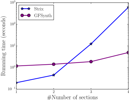
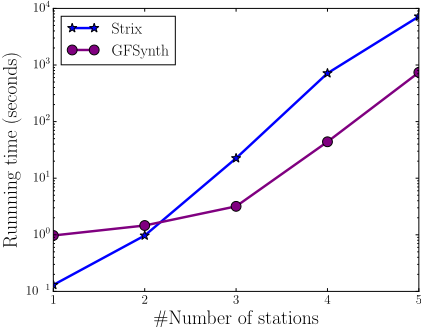
Figure 1 and Figure 2 show the running time of GFSYNTH and STRIX on both benchmarks, respectively. The x-axis indicates the value of the scalable parameter n for each benchmark. The y-axis is in log scale. Results of cases on which both tools failed are not shown. For benchmark Finding Nemo, in small cases where n ≤ 2, there is no large gap in the time cost. However, as n grows, the time cost of GFSYNTH increases linearly, while the time cost of STRIX increases exponentially. Regarding benchmark Workstation Resupply, the exponential gap is not so obvious. Nevertheless, as the benchmark grows, STRIX almost always takes around 10 times longer than GFSYNTH. STRIX also failed for n = 5.

Discussions. Looking deeper into GFSYNTH, we observed that on those cases where GFSYNTH fails, the automata can not be constructed by the MONA library employed by SYFT for automata construction from LTLf . There has been various studies on LTLf -to-automata translation. Possibly the most successful attempt is the decompositional approach presented in [Bansal et al., 2020]. For future work, we will take this approach into account to improve GFSYNTH.

Acknowledgments

Research partially supported by the ERC Advanced Grant WhiteMech (No. 834228), the EU ICT-48 2020 project TAILOR (No. 952215), NSF grants IIS-1527668, CCF-1704883, IIS-1830549, and an award from the Maryland Procurement Office.