A Runtime Analysis of Typical Decomposition Approaches in MOEA/D Framework for Many-objective Optimization Problems

1 Introduction

Multi-objective optimization problems (MOPs) involve optimizing multiple conflicting objective functions simultaneously. MOPs with at least four objectives widely exist in real-word applications and are referred to as manyobjective optimization problems (MaOPs) [Li et al., 2015a]. Multi-objective evolutionary algorithms (MOEAs) are popular methods for handling MOPs, and can be roughly classified into three categories, i.e., domination-based, indicator-based and decomposition-based [Trivedi et al., 2017].

Domination-based MOEAs, such as NSGA-II [Deb et al., 2002], are quite effective in solving low-dimensional MOPs. But they often suffer from dramatic performance degeneration when handling MaOPs, because of insufficient selection pressure toward the Pareto front [Li et al., 2015b]. Due to the computation time of indicators rapidly increasing with the number of objectives, indicator-based MOEAs are largely restricted to solve MaOPs [Deng and Zhang, 2019]. Although these defects have been alleviated in some researches, (e.g., [Yuan et al., 2016] and [Rostami and Neri, 2017]), decomposition-based MOEAs have attracted the most attention and are very popular for solving MaOPs in the past decade [Trivedi et al., 2017].

∗Corresponding author

Decomposition-based MOEAs have been implemented in [Ishibuchi and Murata, 1998]. They became popular after [Zhang and Li, 2007] proposed the classic MOEA/D framework. In the MOEA/D framework, an MaOP is first decomposed into a number of scalar subproblems according to the used decomposition approach and a set of weight vectors, then all subproblems are solved in parallel and collaboratively by using an evolutionary algorithm (EA). Decomposition approach is an important component in MOEA/D framework, since it determines the analytical expression formula of the subproblems and guides the evolutionary search [Wang et al., 2020]. The typical decomposition approaches used in MOEA/D framework are weighted sum (WS), Tchebycheff (TCH) [Das and Dennis, 1998], and penalty-based boundary intersection (PBI) [Zhang and Li, 2007]. Many researches have developed novel decomposition approaches based on them, e.g., [G´omez and Coello, 2017; Luque et al., 2020].

Running time or runtime analysis is an essential and powerful theory aspect to understand the work principles of EAs [Qian et al., 2019]. Li et al. [2016] presented a runtime analysis of a simple algorithm based on MOEA/D framework, which only applies mutation operator to create offspring. Later, Huang et al. [2020] extended the analysis to the universal case that selects mutation or crossover to create offspring with a control parameter. Recently, a runtime analysis of a simple MOEA/D using somatic contiguous hypermutation operators [Jansen and Zarges, 2011] to create offspring was presented in [Huang and Zhou, 2020]. These theoretical studies have revealed some important optimization behaviors of decomposition-based MOEAs. However, they only consider the case of using TCH approach and the number of objectives in their analyzed problems is at most four.

This paper presents a runtime analysis for the convergence ability of using three typical decomposition approaches in a basic MOEA/D on optimizing benchmark MaOPs. Specifically, we analyze and compare the expected runtime of a basic decomposition-based MOEA with WS, TCH or PBI finding an optimal solution for any subproblem of two benchmark MaOPs, namely mLOTZ and mCOCZ [Laumanns et al., 2004]. Note that in the two problems, m represents the number of the objectives and it is a variable. They have been served as benchmark problems for theoretical analyses of MOEAs, e.g., [Laumanns et al., 2004; Bian et al., 2018].

The theoretical results show that using WS, the algorithm can always find an optimal solution for any subproblem of mLOTZ and mCOCZ in polynomial expected runtime O( n2 log n m ) and Θ(n logn), respectively. When using TCH, the expected lower bounds of the algorithm are Ω( n2 m ) and Ω(n logn), respectively. But the expected upper bounds are O(n2mm/2 ) and O( nm/2+1 m ), respectively. When using PBI, the expected runtime is dependent on the setting of the penalty parameter θ. In the best case (i.e., θ = 0), they are equal to that of using WS. In the worst case, the algorithm cannot find an optimal solution for some subproblems if θ is set too large. Moreover, our analyses discover an obvious shortcoming of using WS, i.e., the optimal solutions of different subproblems are easily corresponding to the same solution. In addition, our analyses indicate that increasing parameter θ is harmful for faster converging to the PF when using PBI, but it can alleviate the shortcoming of WS. This theoretical study reveals some important optimization behaviors of using the three typical decomposition approaches in MOEA/D for solving MaOPs, and may be helpful for designing more efficient MOEAs in future research.

2 Preliminaries

2.1 Analyzed Problems

Formally, a maximization MOP can be defined as follows:

where x is the decision variable, X is the decision space, F : X → Rm consists of m objective functions and Rm is the objective space. For x1, x2 ∈ X, we say that x1 weakly dominates x2, denoted as x1 ⪰ x2, if fi(x1) ≥ fi(x2) for all i = 1, . . . ,m. If x1 ⪰ x2 and F(x1) ̸= F(x2), we say that x1 dominates x2, denoted as x1 ≻ x2. A solution x∗ ∈ X is Pareto optimal if there is no solution x ∈ X such that x ≻ x∗ . The set of all Pareto optimal solutions is called Pareto-optimal set or Pareto set (PS) and the set of objective vectors corresponding to the PS is called Pareto front (PF).

Let x be a bit string of length n, i.e., x ∈ {0, 1}n , and x[i] denote the value of the i-th bit of x for i = 1, 2, . . . , n. The benchmark MaOPs (i.e., mLOTZ and mCOCZ [Laumanns et al., 2004]) analyzed in this paper can be defined as follows.

Definition 1 (mLOTZ). The pseudo-Boolean function mLOTZ : {0, 1}n → Nm is defined as follows:

where

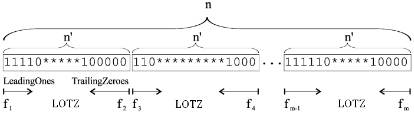
m is an even number, n′ is a natural number and n′ = 2n m . Definition 2 (mCOCZ). The pseudo-Boolean function mCOCZ : {0, 1}n → Nm is defined as follows:

where

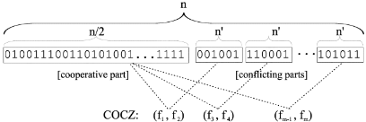
m is an even number, n′ is a natural number and n′ = nm .

Note that all objective functions in mLOTZ and mCOCZ require to be maximized simultaneously. For mLOTZ, it is a concatenation of m2 LOTZ (leading ones trailing zeros) [Laumanns et al., 2004]. There are m2 conflicting parts in the search space, as shown in Figure 1 [Laumanns et al., 2004]. For mCOCZ, it is a combination of m2 COCZ [Laumanns et al., 2004]. There are cooperative and conflicting parts in the solution space, as shown in Figure 2 [Laumanns et al., 2004].

2.2 Decomposition Approaches

In MOEA/D, an MOP is first decomposed into a number of scalar optimization subproblems according to the decomposition approach and a set of weight vectors. WS, TCH and PBI are classic decomposition approaches used in MOEA/D framework. Given a maximization MOP and a weight vector λ = (λ1, . . . , λm) satisfying λi ≥ 0 for i = 1, . . . ,m and ∑mi=1 λi = 1, the subproblems generated by WS, TCH and PBI are shown in Eq. (2), Eq. (3) and Eq. (4), respectively.

Algorithm 1 A simple decomposition-based MOEA

Input: An MOP with m objectives, stop criterion, weight vectors {λ1 , . . . , λN } and neighbor size T .

Output: A candidate Pareto optimal solution set P .

• 1: Initialization: A candidate Pareto optimal solution set P = ∅. Decompose the original MOP into N scalar subproblems according to the used decomposition approach and weight vectors {λ1 , . . . , λN }. For each subproblem g(x|λk ), k = 1, 2, . . . ,N, select the T closest subproblems to form its neighbor set Bk according to the Euclidean distance between their weight vectors. Generate solution xk ∈ {0, 1}n uniformly at random for each g(x|λk ). Let Sk denote the set of solutions corresponding to the subproblems in Bk.
• 2: while stop criterion is not satisfied do
• 3: for each subproblem g(x|λk ), k = 1, 2, . . . , N do
• 4: Reproduction: create offspring yk by randomly flipping one bit in xk.
• 5: Update Sk: for each solution xj in Sk, if g(yk|λj ) is not worse then g(xj|λj ), replace xj with yk.
• 6: Update P: remove all solutions weakly dominated by yk from P . If yk is not dominated by any solution in P, add yk into P.
• 7: end for
• 8: end while

where z∗ = (z∗ 1 , . . . , z ∗m) denotes the reference point, i.e., z∗ i =max{fi(x)|x ∈ X}.

where z∗ has the same meaning with Eq. (3), θ > 0 is the penalty parameter and

As shown above, for a given weight vector, different decomposition approaches transform an MOP into different scalar subproblems and they largely affect the optimization.

2.3 Analyzed Algorithm

After decomposition, MOEA/D framework controls a population of size N to cooperatively solve all subproblems in parallel via the neighborhood-based coevolution. The analyzed algorithm in this paper is summarized in Algorithm 1. Note that Algorithm 1 can be instantiated by using different decomposition approaches in the initialization (line 1). This paper mainly concerns on the expected runtime of Algorithm 1 with WS, TCH or PBI approach converging to an optimal solution of any subproblem for mLOTZ and mCOCZ. To simplify the observation, the one-bit mutation operator [Zhou et al., 2019], which flips a randomly chosen bit of the parent in a mutation, is used to create offspring in Algorithm 1.

3 Runtime Analysis

Since we mainly focus on the convergence speed of using the three decomposition approaches, we afterward assume that λi=1,2,...,m > 0 holds for weight vector λ = (λ1, . . . , λm) and set the neighbor size T = 1 for the sake of simplicity.

3.1 Analysis onWS

Recall that mLOTZ is a concatenation of m2 LOTZ problems (see Figure 1). For ease of expression, we call the j-th LOTZ as component/part j in the following analysis. Let 1i 0h-i denote the bit-string of length h with i leading 1-bits and h-i trailing 0-bits.

Lemma 1. For mLOTZ, if Algorithm 1 uses WS decomposition approach, all components in the optimal solution for any subproblem are in the form of 1i 0 2n m -i .

Proof. Given weight vector λ = (λ1, . . . , λm), according to Eq. (2) the subproblem generated by WS for mLOTZ is

where fk(x) equals the number of leading 1-bits in component ⌈ k2 ⌉ if k is odd, otherwise it equals the number of trailing 0-bits in this component (see Definition 1).

We first show that all components in any optimal solution are in the form of 1i 0 2n m -i . Otherwise there is at least a component j in it in the form of 1l1 0#10l2 , where # denotes the wildcard string. If the mutation operator flips the leftmost 0-bit or the rightmost 1-bit, it becomes 1l1+1 0#10l2 or 1l1 0#10l2+1 . The function value of the offspring on objective f2j-1 or f2j is larger than its parent, and its function values on other objectives are unchanged. Thus, Algorithm 1 finds a better function value for Eq. (5). This contradicts with the assumption that the current solution is an optimum.

Furthermore, we consider the two values in weight vector λ = (λ1, . . . , λm) related to component j, i.e., λ2j-1 and λ2j. We have λ2j-1 > λ2j, λ2j-1 < λ2j or λ2j-1 = λ2j. Let xj = 1i 0 2n m -i , i = 0 . . . , 2n m - 1 denote component j in the current solution.

If λ2j-1 > λ2j and the mutation operator flips the leftmost 0-bit in xj , it becomes yj = 1i+1 0 2n m -i-1 . The offspring is an improved solution for Eq. (5), because of λ2j-1 · f2j-1(yj )+λ2j · f2j(yj )-λ2j-1 · f2j-1(xj )-λ2j · f2j-1(xj ) = λ2j-1 - λ2j > 0. By analogy, Algorithm 1 can repeatedly create an improved solution for Eq. (5) by flipping the leftmost 0-bit in xj into 1-bit until it becomes the optimal form 1 2n m . Similarly, we know that if λ2j-1 < λ2j, Algorithm 1 can repeatedly create an improved solution for Eq. (5) by flipping the rightmost 1-bit into 0-bit until it becomes 0 2n m .

If λ2j-1 = λ2j , for any two bit-strings s1 = 1i1 0 2n m -i1 and s2 = 1i2 0 2n m -i2 , we have λ2j-1 · f2j-1(s1) + λ2j · f2j (s1) - λ2j-1 · f2j-1(s2) -λ2j · f2j(s2) = 0. Thus, in this case all bit-strings in the form of 1i 0 2n m -i have the same contribution to the function value of Eq. (5) and are optimal form.

Theorem 1. For mLOTZ, using WS decomposition approach, the lower bound and upper bound of expected runtime of Algorithm 1 finding an optimal solution for any subproblem are Ω(max{ n2 m , n log n}) and O( n2 log m m ), respectively.

Proof. First of all, the expectedHamming distance of any initial solution from an optimal solution is E(d) = n · 12 = n2 . Recall that all initial solutions are generated from {0, 1}n uniformly at random, and all components in an optimal solution are in the form of 1i 0 2n m -i . By Chernoff bound, we have Pr(E(d) ≤ n4 ) ≤ e-Θ(n) . Thus, the expected number of bits in any initial solution needed to be corrected before it becomes an optimal one is at least n4 with probability 1-e-Ω(n) .

Moreover, given any component, if it is not in the form of 1i 0 2n m -i , Algorithm 1 can create an improved offspring by flipping the leftmost 0-bit or the rightmost 1-bit in them (refer to the proof of Lemma 1). If it is in the form of 1i 0 2n m -i but not an optimal form, Algorithm 1 can obtain an improvement by flipping either the leftmost 0-bit or the rightmost 1-bit in them. Thus, in a generation the probability of Algorithm 1 creating an improved solution for Eq. (5) is at least hn and at most 2h n , where h denotes the number of components that are not in its optimal form in the current solution.

By using the optimistic assumption that the n4 bits needed to be corrected are done with the highest possible probability, i.e., 2h n = mn , the expected runtime of Algorithm 1 finding an optimal solution for Eq. (5) is lower bounded by n4 · nm = Ω( n2 m ). In addition, according to the proof of Theorem 5.11 in [Jansen, 2013], we know that the n4 bits needed to be corrected have not been done with constant probability within (n - 1) logn fitness evaluations. Thus, the lower bound of expected runtime is Ω(max{ n2 m , n log n}).

To derive the upper bound, we need to consider the worst case that all bits in the initial solution are needed to be corrected and they are done by using the maximum possible probability with minimum quantity. Observe that in this case Algorithm 1 can create improved offspring with the highest possible probability, namely mn , until the number of components that are not in form of 1i 0 2n m -i is less than m2 . This implies that at least all bits in a component are done with this probability and the number of Algorithm 1 creating improved solution with the highest probability is at least 2n m . Similarly, we know that in the worst case the number of Algorithm 1 creating improved solution with probability m-1 n is also 2n m , and so on until 1n . Therefore, the expected runtime of Algorithm 1 finding an optimal solution for Eq. (5) is upper bounded by ∑m/2 j=1 2n m · nj ≤ ∑mj=1 2n m · nj = O( n2 logm m ).

Lemma 2. For mCOCZ, using WS approach, the lower bound of expected runtime of Algorithm 1 finding an optimal solution for every subproblem is Ω(n log n).

For mCOCZ, the subproblem generated by WS for weight vector λ = (λ1, . . . , λm) is

where fk(x) is shown in Definition 2.

Observe that for Eq. (6), all fk(x) increase when increasing the number of 1-bits in the first half of x (the cooperative part). This implies that a necessary condition of an initial solution becoming an optimum is that the first n2 bits are transformed into 1-bits. Thus, we can conclude this result according to the proof of Theorem 5.11 in [Jansen, 2013]. We omit the detailed proof for the sake of space limitation.

Lemma 3. For mCOCZ, using WS approach, the upper bound of expected runtime of Algorithm 1 finding an optimal solution for any subproblem is O(n log n).

Proof. Let i < n2 denote the number of 1-bits in the first half of the initial solution. In a generation, if one of the i 0-bits is flipped, Algorithm 1 obtains an improvement for Eq. (6). This event happens with probability in . Thus, the expected runtime of Algorithm 1 transforming all bits in the cooperative part into 1-bits is upper bounded by ∑n/2-1 i=1 ni = O(n logn).

We next consider the conflicting part. Given any component j, similar to analysis in the proof of Lemma 1, we know that its optimal form is 1 nm if λ2j-1 > λ2j and is 0 nm if λ2j-1 < λ2j. Otherwise, it can be any bit-string with length nm . Let dj denote the Hamming distance of the current component j from its optimal form. Observe that in a generation Algorithm 1 can create an improved offspring for Eq. (6) by flipping one of the dj wrong bits in this part. Thus, in a generation Algorithm 1 finds an improved solution for Eq. (6) with probability is d1+···+dm/2 n . Note that 1 ≤ ∑m2 i=1 dj ≤ n2 holds if the current solution is not an optimum. Therefore, Algorithm 1 transforms the conflicting part into an optimal form in expected runtime ∑n2 i=1 ni = O(n logn).

Combining Lemma 2 and Lemma 3, we have Theorem 2.

Theorem 2. For mCOCZ, using WS decomposition approach, the expected runtime of Algorithm 1 finding an optimal solution for any subproblem is Θ(n log n).

3.2 Analysis on TCH

Lemma 4. For mLOTZ, using TCH approach, the expected lower bound of Algorithm 1 finding an optimal solution for any subproblem is Ω( n2 m ) with probability 1 - e-Ω( nm ) .

Proof. For mLOTZ, the reference point is z∗ = ( 2n m , . . . , 2n m ). Given weight vector λ = (λ1, . . . , λm), according to Eq. (3) the subproblem produced by TCH is

where fk(x) is the same as that in Eq (5).

Observe that Eq. (7) requires to find a x∗ such that x∗ = arg minx∈X {maxk=1...,m{λk ( 2n m -fk(x))}}. For any x, let Vmax(x) :=maxk=1,...,m{λk ( 2n m -fk(x))} and Imax(x) = {k|λk ( 2n m - fk(x)) ≥ Vmax(x)}. Note that for mLOTZ there is no solution that can increase multiple function objective values simultaneously. Thus, in a generation Algorithm 1 creates an improved offspring x′ from parent x if and only if: (1) |Imax(x)| = 1 (denote by k′ the element in Imax(x)); (2) the one-bit mutation flipping one bit in the component ⌈ k′ 2 ⌉ of x such that fk′(x′ ) > fk′(x), i.e., either the leftmost 0-bit or the rightmost 1-bit in the part ⌈ k′ 2 ⌉ is flipped (denoted as event E1). Thus, in a generation event E1 happens with probability at most 2n and the expected runtime of Algorithm 1 obtaining such an improvement is Ω(n).

We next show that the expected number of improvements for finding an optimal solution is Ω( nm ). First, for any optimal solution of Eq. (7), the part ⌈ k′ 2 ⌉ must be in the form of 1i 0 2n m -i . Otherwise, it is 1l1 0#10l2 . If the rightmost 1-bit is flipped, the function value on objective fk′ is increased. This means that a better solution is found, which contradicts with the assumption. Second, according to analysis in the proof of Theorem 1, we have that to transform any component into the form of 1i 0 2n m -i , the number of bits that needed to be corrected is at least n 2m with probability 1 - eΩ( nm ) .

Therefore, with probability 1-e-Ω( nm ) the expect runtime of Algorithm 1 using TCH approach finding an optimal solution for any subproblem is Ω(n) · Ω( nm ) = Ω( n2 m ).

Lemma 5. For mLOTZ, using TCH approach, the expected upper bound of Algorithm 1 finding an optimal solution for any subproblem is O(n2mm/2-2 ).

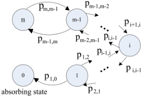
Proof. We consider the random process that Algorithm 1 obtains an improved offspring starting from solution x with |Imax(x)| = i, i ∈ {1, . . . ,m}. Let pi,i-1 be the probability of Algorithm 1 creating an offspring x′ from x such that |Imax(x′ )| = i - 1. Observe that to delete an element from Imax(x), Algorithm 1 needs to flip either the leftmost 0bit or the rightmost 1-bit in the related component. So there are exactly i bits which flipping one of them can decrease |Imax(x)| by one. Thus, we have pi,i-1 = in . However, in this situation Algorithm 1 can also create an offspring y from x such that |Imax(y)| = i + 1, if it flips one of m- i bits in x leading to the value of an objective not in Imax(x) increase to Vmax(x) (denoted as event E2). The probability of event E2 is m-i n . Note that y is also accepted to replace x in such a mutation, because it has the same fitness value with the parent. In other words, to obtain an improved solution for Eq. (7), Algorithm 1 needs to pass through a plateau including at most m points, which is equivalent to reaching the absorbing state of Markov chain shown in Figure 3. The transition probability matrix P of the Markov chain is

Let Ti denote the expected runtime of Algorithm 1 reaching the absorbing sate from state i = 0, 1, . . . , m, and use p-i and p+i as shorthand for pi,i-1 and pi,i+1 in P, respectively. According to Corollary 2 in [Zhou et al., 2009], we have

p-m-1-(l+1) ( 1 p-m-(l+1) + gl ). By Eq. (8), the expected runtime of Algorithm 1 obtaining an improved solution for Eq. (7) from the current one is upper bounded by Tm = T0 + ∑mi=1 1 p-i + ∑m-2 j=0 gj ≤ O(nmm/2-1 ).

Note that for any weight vector, the function value of any objective contains at most 2n m members, since there are 2n m bits in any component. Thus, using TCH approach, the expect runtime of Algorithm 1 finding an optimal solution for any subproblem is O(nmm/2-1 ) · O( nm ) = O(n2mm/2-2 ).

Combining Lemma 4 and Lemma 5, we have Theorem 3.

Theorem 3. For mLOTZ, using TCH decomposition approach, the lower bound and upper bound of expected runtime of Algorithm 1 finding an optimal solution for any subproblem are Ω( n2 m ) and O(n2mm/2-2 ), respectively.

Lemma 6. For mCOCZ, using TCH approach, the lower bound of expected runtime of Algorithm 1 finding an optimal solution for any subproblem is Ω(n log n).

For mCOCZ, the reference point is z∗ = ( n2 + nm , . . . , n2 + nm ). According to Eq. (3), the scalar subproblem produced by TCH for weight vector λ = (λ1, . . . , λm) is

where fk(x) is shown in Definition 2. The main idea of proving this lemma is the same as that of Lemma 2, since Eq. (6) and Eq. (9) have the same property in the cooperative part.

Lemma 7. For mCOCZ, using TCH approach, the upper bound of expected runtime of Algorithm 1 finding an optimal solution for any subproblem is O( nm/2+1 m ).

Proof. First, similar to the proof of Lemma 3, we know that Algorithm 1 transforms the first n2 bits into 1-bits in expected runtime O(n logn). We next consider the expected runtime to handle the conflicting part after this phase. We claim that for Eq. (9), |Imax(x)| ≤ m2 holds for any non-optimal solution x. Recall that there are m2 components in the conflicting part. If |Imax(x)| > m2 , there are at least two elements in the same component, i.e., existing a j ∈ {1, 2, . . . , m2 } such that λ2j-1 ( n2 + nm -f2j-1(x)) = λj ( n2 + nm -fj(x)). Observe that f2j-1(x) and f2j(x) are conflicting. Thus, f2j-1(x) will be decreased when f2j(x) increasing and vice verse. Hence, the maximum of them cannot be decreased by flipping any bits in x. Therefore, the function value of Eq. (9) is at least λ2j-1 ( n2 + nm - f2j-1(x)) and x is an optimal solution.

Suppose that |Imax(x)| = h holds for the current solution x. Let vector vd denote the differences between 1-bits in all conflicting component of x and the optimal solution, and let i be the minimum value in vd. Note that all values in vd are integers. This means that for each component (or element) in Imax(x), there are at least i 1-bits or 0-bits which flipping one of them can decrease the number of elements in Imax(x) by one. And for any component not in Imax(x), there are at most ( nm - i) 1-bits or 0-bits which flipping one of them can increase the number of elements in Imax(x) by one. Thus, in a generation, the probabilities of Algorithm 1 creating and accepting an offspring x′ from x such that |Imax(x′ )| is h-1 or h+1 are h·i n ≥ hn and (m/2-h)·(n/m-i) n ≤ m-2h 2m , respectively. Thus, the transition probability matrix pm2 +1, m2 +1 of finding an improved solution for the subproblem is

where pi,i = 1-p+i -p-i for i = 1, 2, . . . , m2 -1. By using the same argument in the proof of Lemma 5,

Note that for mCOCZ the number of 0-bits or 1-bits in any conflicting part is at most nm . Thus, the expected runtime of Algorithm 1 finding an optimal solution for Eq. (9) is

Combining Lemma 6 with Lemma 7, we have Theorem 4. Theorem 4. For mCOCZ, using TCH decomposition approach, the lower bound and upper bound of expected runtime of Algorithm 1 finding an optimal solution for any subproblem are Ω(n log n) and O( nm/2+1 m ), respectively.

From the proofs of Lemmas 5 and 7, we know that the exponential expected upper bounds of using TCH are caused by the fact that it introduces many plateaus of size Θ(m) into the function landscape of some subproblems, and such a situation is likely to be encountered in handling other MaOPs.

3.3 Analysis on PBI

Theorem 5. For mLOTZ and mCOCZ, Algorithm 1 using PBI finds an optimal solution for any subproblem in expected runtime Ω(max{ n2 m , n log n}) and Ω(n log n), respectively.

Proof. First, if the penalty parameter θ is set to 0, Eq. (4) (subproblem generated by PBI for weight vector λ) becomes

Note that for any MOP and weight vector λ, ∑mk=1 λkz∗ k and ‖λ‖ are fixed. Thus, the optimization of Eq. (10) is equivalent to finding x∗ = argmax ∑mk=1 λkfk(x), which equals Eq. (2) (subproblem generated by WS). Second, with increasing parameter θ, the penalty of individual deviating from weight vector λ, namely the emphasis on diversity, is increased. As a result, some improved offspring for the case of using WS, which deviate from λ by too large an amount, will not be accepted if using PBI since their fitness values become worse (see Eq. (4)) in this situation. Thus, in any generation the probability of Algorithm 1 finding an improved offspring is at most that of using WS and the theorem is proven.

Chen et al. [2019] proved that for any MOP and weight vector, the optimization of subproblem generated by WS is equivalent to that of by PBI with a specific setting of θ. Unfortunately, this does not hold in reverse. In fact, if θ is set too large, Algorithm 1 will never find an optimal solution for some subproblems, because it only accepts offspring that increase the function values of multiple objectives (i.e., flipping multiple bits in the parent). This is impossible for the one-bit mutation. If Algorithm 1 applies the standard bit mutation (SBM) [Doerr and Neumann, 2019] (also called bit-wise mutation [Zhou et al., 2019]), which often flips each bit in the parent with independent probability 1n , it can flip multiple bits in a mutation. But the convergence speed is rather slow since SBM flips j bits in a mutation with probability O( 1 nj ).

In summary, Algorithm 1 using WS can find an optimal solution for any subproblem of analyzed problems in polynomial expected runtime. But such a result may be not true for the case of using TCH or PBI. Moreover, the proofs of Lemmas 1 and 3 imply that the optimal solutions of different subproblems are easily corresponding to the same solution if using WS. And the proof of Theorem 5 indicates that increasing the parameter θ in PBI approach is harmful for faster converging to the PF, but it can increase the diversity.

4 Conclusions

This paper theoretically investigates the convergence speed of using the typical WS, TCH and PBI decomposition approaches in the MOEA/D framework for solving MaOPs. The results show that using WS, the algorithm can find an optimal solution for any subproblem of analyzed problems in polynomial expected runtime. When using TCH or PBI, the algorithm needs at least exponential expected runtime for some subproblems. Moreover, our analyses discover an obvious shortcoming of usingWS, that is, the optimal solutions of different subproblems are easily corresponding to the same solution. And decreasing the penalty parameter in PBI is good for faster converging to the PF, but it may lose the diversity.

Acknowledgements

This work is supported by the National Natural Science Foundation of China (61773410) and Microsoft Research Asia.