
RCA: A Deep Collaborative Autoencoder Approach for Anomaly Detection
Proceedings of the Thirtieth International Joint Conference on Artificial Intelligence. Main Track. Pages 1505-1511.
https://doi.org/10.24963/ijcai.2021/208
Keywords
- Machine Learning: Unsupervised Learning
- Data Mining: Anomaly/Outlier Detection
Abstract
Unsupervised anomaly detection plays a crucial role in many critical applications. Driven by the success of deep learning, recent years have witnessed growing interests in applying deep neural networks (DNNs) to anomaly detection problems. A common approach is using autoencoders to learn a feature representation for the normal observations in the data. The reconstruction error of the autoencoder is then used as outlier scores to detect the anomalies. However, due to the high complexity brought upon by the over-parameterization of DNNs, the reconstruction error of the anomalies could also be small, which hampers the effectiveness of these methods. To alleviate this problem, we propose a robust framework using collaborative autoencoders to jointly identify normal observations from the data while learning its feature representation. We investigate the theoretical properties of the framework and empirically show its outstanding performance as compared to other DNN-based methods. Our experimental results also show the resiliency of the framework to missing values compared to other baseline methods.
- [Aggarwal and Sathe, 2017] Charu C Aggarwal and Saket Sathe. Outlier ensembles: An introduction. Springer, 2017.
- [An and Cho, 2015] Jinwon An and Sungzoon Cho. Varia- tional autoencoder based anomaly detection using recon- struction probability. Special Lecture on IE, 2(1):1-18, 2015.
- [Chandola et al., 2009] Varun Chandola, Arindam Banerjee, and Vipin Kumar. Anomaly detection: A survey. ACM computing surveys (CSUR), 41(3):1-58, 2009.
- [Chen et al., 2001] Yunqiang Chen, Xiang Sean Zhou, and Thomas S Huang. One-class svm for learning in image retrieval. In Proceedings 2001 International Conference on Image Processing (Cat. No. 01CH37205), volume 1, pages 34-37. IEEE, 2001.
- [Emmott et al., 2015] Andrew Emmott, Shubhomoy Das, Thomas Dietterich, Alan Fern, and Weng-Keen Wong. A meta-analysis of the anomaly detection problem. arXiv preprint arXiv:1503.01158, 2015.
- [Han et al., 2018] Bo Han, Quanming Yao, Xingrui Yu, Gang Niu, Miao Xu, Weihua Hu, Ivor Tsang, and Masashi Sugiyama. Co-teaching: Robust training of deep neural networks with extremely noisy labels. In Advances in neural information processing systems, pages 8527-8537, 2018.
- [Jiang et al., 2017] Lu Jiang, Zhengyuan Zhou, Thomas Le- ung, Li-Jia Li, and Li Fei-Fei. Mentornet: Learning data- driven curriculum for very deep neural networks on cor- rupted labels. arXiv preprint arXiv:1712.05055, 2017.
- [Kingma and Welling, 2013] Diederik P Kingma and Max Welling. Auto-encoding variational bayes. arXiv preprint arXiv:1312.6114, 2013.
- [Kumar et al., 2010] M Pawan Kumar, Benjamin Packer, and Daphne Koller. Self-paced learning for latent variable models. In Advances in Neural Information Processing Systems, pages 1189-1197, 2010.
- [Liu et al., 2008] Fei Tony Liu, Kai Ming Ting, and Zhi-Hua Zhou. Isolation forest. In 2008 Eighth IEEE International Conference on Data Mining, pages 413-422. IEEE, 2008.
- [Liu et al., 2019] Yezheng Liu, Zhe Li, Chong Zhou, Yuanchun Jiang, Jianshan Sun, Meng Wang, and Xiang- nan He. Generative adversarial active learning for unsu- pervised outlier detection. IEEE Transactions on Knowl- edge and Data Engineering, 2019.
- [Pedregosa et al., 2011] F. Pedregosa, G. Varoquaux, A. Gramfort, V. Michel, B. Thirion, O. Grisel, M. Blon- del, P. Prettenhofer, R. Weiss, V. Dubourg, J. Vanderplas, A. Passos, D. Cournapeau, M. Brucher, M. Perrot, and E. Duchesnay. Scikit-learn: Machine learning in Python. Journal of Machine Learning Research, 12:2825-2830, 2011.
- [Rayana, 2016] Shebuti Rayana. ODDS library. http://odds. cs.stonybrook.edu, 2016. Accessed: 2020-09-01. Link
- [Ruff et al., 2018] Lukas Ruff, Robert Vandermeulen, Nico Goernitz, Lucas Deecke, Shoaib Ahmed Siddiqui, Alexan- der Binder, Emmanuel Müller, and Marius Kloft. Deep one-class classification. In International conference on machine learning, pages 4393-4402, 2018.
- [Sakurada and Yairi, 2014] Mayu Sakurada and Takehisa Yairi. Anomaly detection using autoencoders with non- linear dimensionality reduction. In Proceedings of the MLSDA 2014 2nd Workshop on Machine Learning for Sensory Data Analysis, pages 4-11, 2014.
- [Shah et al., 2020] Vatsal Shah, Xiaoxia Wu, and Sujay Sanghavi. Choosing the sample with lowest loss makes sgd robust. arXiv preprint arXiv:2001.03316, 2020.
- [Shen and Sanghavi, 2018] Yanyao Shen and Sujay Sang- havi. Learning with bad training data via iterative trimmed loss minimization. arXiv preprint arXiv:1810.11874, 2018.
- [Srivastava et al., 2014] Nitish Srivastava, Geoffrey Hinton, Alex Krizhevsky, Ilya Sutskever, and Ruslan Salakhutdi- nov. Dropout: a simple way to prevent neural networks from overfitting. The journal of machine learning re- search, 15(1):1929-1958, 2014.
- [Vincent et al., 2010] Pascal Vincent, Hugo Larochelle, Is- abelle Lajoie, Yoshua Bengio, and Pierre-Antoine Man- zagol. Stacked denoising autoencoders: Learning use- ful representations in a deep network with a local de- noising criterion. Journal of machine learning research, 11(Dec):3371-3408, 2010.
- [Zhang et al., 2016] Chiyuan Zhang, Samy Bengio, Moritz Hardt, Benjamin Recht, and Oriol Vinyals. Understand- ing deep learning requires rethinking generalization. arXiv preprint arXiv:1611.03530, 2016.
- [Zhao et al., 2019] Yue Zhao, Zain Nasrullah, and Zheng Li. Pyod: A python toolbox for scalable outlier detection. arXiv preprint arXiv:1901.01588, 2019.
- [Zhou and Paffenroth, 2017] Chong Zhou and Randy C Paf- fenroth. Anomaly detection with robust deep autoen- coders. In Proceedings of the 23rd ACM SIGKDD Inter- national Conference on Knowledge Discovery and Data Mining, pages 665-674, 2017.
- [Zong et al., 2018] Bo Zong, Qi Song, Martin Renqiang Min, Wei Cheng, Cristian Lumezanu, Daeki Cho, and Haifeng Chen. Deep autoencoding gaussian mixture model for unsupervised anomaly detection. 2018.
References were extracted automatically from the PDF and may contain errors.
Full text extracted automatically from the PDF; figures, tables and equations may differ. The PDF is the version of record.
1 Introduction
Anomaly detection (AD) is the task of identifying unusual or abnormal observations in the data. It has a wide range of applicability, from credit fraud detection to medical diagnosis. Current AD approaches can be divided into supervised or unsupervised learning methods. Supervised AD requires labeled examples to train the AD models whereas unsupervised AD, which is the focus of this paper, does not require label information but assumes there are more normal than anomalous instances in the data [Chandola et al., 2009]. Deep autoencoders are one of the most widely used unsupervised AD methods [Chandola et al., 2009; Sakurada and Yairi, 2014; Vincent et al., 2010]. An autoencoder compresses the original data by learning its hidden representation in a way that minimizes the reconstruction loss. It is based on the assumption that normal observations are easier to compress than anomalies. Unfortunately, such an assumption does not generally hold for DNNs, which are often over-parameterized and have the capability to fit well even to the anomalies [Zhang et al., 2016]. Thus, the DNN-based unsupervised AD methods must consider the trade-off between model capacity and overfitting to the anomalies to achieve good performance.
∗Contact Author
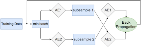
Our work is motivated by recent progress on robustness of DNNs for noisy labeled data by learning the weights of the samples during training [Jiang et al., 2017; Han et al., 2018]. For unsupervised AD, our goal is to learn the weights in such a way that normal observations are assigned higher weights than anomalies when calculating reconstruction error. The weights can be used to reduce the influence of anomalies when updating the model for learning a feature representation of the data. However, existing approaches for weight learning are inapplicable to unsupervised AD as they require label information. To address this challenge, we propose a robust collaborative autoencoders (RCA) method that trains a set of autoencoders in a collaborative fashion and jointly learns their model parameters and sample weights. Specifically, given a mini-batch, each autoencoder would learn a feature representation and selects a subset of the samples with lowest reconstruction errors. By discarding samples with high reconstruction errors, the learning algorithm focuses more on fitting the clean data, thereby reducing its risk of memorizing anomalies. However, by selecting only easy-to-fit samples, this may lead to premature convergence of the algorithm without sufficient exploration of the loss surface. To address this issue, the proposed approach selects samples from each autoencoder and exchange them between them, to update their model weights. The sample selection and exchanging procedures are illustrated in Figure 1. During the testing phase, we apply a dropout mechanism to produce multiple output predictions for each test point by repeating the forward pass multiple times. The ensemble of outputs are then aggregated to obtain a robust estimate of the anomaly score.
The main contributions of this paper are as follows. First, we present a framework for unsupervised deep AD using robust collaborative autoencoders (RCA) to prevent model overfitting due to anomalies. Second, we provide theoretical analysis to understand the mechanism behind RCA. Our analysis shows that the worst-case scenario for RCA is better than conventional autoencoders and provides the conditions under which RCA will detect the anomalies. Third, we show that RCA outperforms state-of-the-art unsupervised AD methods for the majority of the datasets used in this study, even if there are missing values present in the data. In addition, RCA also enhances the performance of more advanced autoencoders such as variational autoencoders in unsupervised AD tasks.
2 RelatedWork
Many methods have been developed over the years for unsupervised AD [Chandola et al., 2009]. Reconstruction-based methods, such as principal component analysis (PCA) and autoencoders, project the input data to a lower-dimensional manifold before transforming them back to the original feature space. The distances between the input and reconstructed data are used as anomaly scores of the data points. [Zhou and Paffenroth, 2017] combined robust PCA with an autoencoder to decompose the data into a mixture of normal and anomaly parts. [Zong et al., 2018] jointly learned a low dimensional embedding and density of the data, using the density of each point as its anomaly score while [Ruff et al., 2018] extended the traditional one-class SVM approach to a deep learning setting. Current deep AD methods cannot prevent the network from incorporating anomalies into their learned representation. One way to address the issue is by assigning a weight to each data point. For example, in self-paced learning [Kumar et al., 2010], the algorithm assigns higher weights to easier-to-classify examples and lower weights to harder ones. This strategy was adopted by other supervised methods for learning from noisy labeled data, including mentornet [Jiang et al., 2017] and co-teaching [Han et al., 2018]. Extending the weight learning methods to unsupervised AD is a key novelty of our work. Theoretical studies on the benefits of choosing samples with smaller loss to drive the optimization algorithm can be found in [Shen and Sanghavi, 2018].
3 Methodology
Let X ∈ Rn×d denote the input data, where n is the number of observations and d is the number of features. Our goal is to classify each xi ∈ X as an anomaly or a normal observation. Let O ⊂ X be the set of true anomalies in the data and ϵ = |O|/n be the anomaly ratio, which is determined based on the amount of suspected anomalies in the data or the proportion the user is willing to inspect and verify.
The RCA framework trains a set of k autoencoders with different initializations. For brevity, we assume k = 2 even though RCA is applicable to more than 2 autoencoders. In each iteration during training, the autoencoders will each apply a forward pass on a mini-batch randomly sampled from the training data and compute the reconstruction error of each
Algorithm 1: Robust Collaborative Autoencoders
input: training data Xtrn, test data Xtst, anomaly ratio ϵ, dropout rate r, decay rate α, and max epoch for training; initialize autoencoders A1 and A2; sample selection β = 1; Training Phase while epoch ≤ max epoch do for minibatch S in Xtrn do ˆS1 ← forward(A1, S, dropout = 0), ˆS2 ← forward(A2, S, dropout = 0); c1 ← sample selection(ˆS1, S, β), c2 ← sample selection(ˆS2, S, β) ; ˆS1 ← forward(A1, S[c2], dropout = r), ˆS2 ← forward(A2, S[c1], dropout = r); A1 ←backprop(ˆS1, S[c2], dropout = r), A2 ← backprop(ˆS2, S[c1], dropout = r) ; end β = max(β - ϵ α × max epoch , 1 - ϵ) end return A∗1 = A1 and A∗2 = A2 ; Testing Phase ξ = []; for i = 1 to v do ξ1= forward(A∗1, Xtst, dropout = r) ; ξ2=forward(A∗2, Xtst, dropout = r) ; ξ.append((ξ1 + ξ2)/2); end return anomaly score = average(ξ) ;data point in the mini-batch. Each autoencoder will then sort the data points according to their reconstruction errors and selects the points with lowest reconstruction error to be exchanged with another autoencoder. This is known as the sample selection step. A back-propagation step is then performed by each autoencoder to update its model parameters using the samples it receives from another autoencoder. Upon convergence, the averaged reconstruction error of each data point is treated as its anomaly score. A pseudocode for RCA with k = 2 autoencoders is shown in Algorithm 1.
3.1 Sample Selection
We present theoretical results to motivate our sample selection approach. First, we demonstrate the robustness of RCA against contamination (anomalies) in training data by showing that RCA converges to a similar solution as if it had been trained on clean (normal) data without anomalies. Next, we show that RCA is better than vanilla SGD when the anomaly ratio is large or when the anomalies are very different from normal data. Finally, we show that RCA will correctly select all the normal points under certain assumption.
Given a mini-batch, Xm ⊂ X, our sample selection procedure chooses a subset of points with lowest reconstruction error as "clean" samples to update the parameters of the autoencoder. The selected points may vary from one iteration to another depending on which subset of points are in the mini-batch and which points have lower reconstruction error within the mini-batch. To avoid discarding the data points prematurely, we use a linear decay function from β = 1 (all points within the mini-batch are chosen) until β = 1 - ϵ to gradually reduce the proportion of selected samples (see last line of training phase in Algorithm 1). The rationale for this approach is that we observe the autoencoders to overfit the anomalies only when the number of training epochs is large.
Let k be the mini-batch size and w be the current parameter of an autoencoder. Our algorithm selects (β × 100)% of the data points with lowest reconstruction errors in the mini-batch to update the autoencoder. Let pi(w) be the probability that a data point with ith smallest reconstruction error (among all n points in the entire dataset) is chosen to update the parameters of the autoencoder. Assuming sampling without replacement, we consider two cases: i ≤ βk and i > βk. In the first case, the data point with ith smallest error will be selected as long as it is in the mini-batch. In the second case, the point is chosen only if it is part of the mini-batch and has among the (βk)-th lowest errors in the mini-batch:
The objective function for the autoencoder with sample selection can thus be expressed as follows:
where f(xi,w) = fi(w) is the reconstruction loss for xi. Suppose Ω(w∗ sr ) is the set of stationary points for ˆ F(w) and Ωi(w∗ ) is the corresponding set of stationary points for each individual loss, fi(w). Let F(w) = ∑i/∈O fi(w) be the "clean" objective function, where anomalies have been excluded from the training data and Ω(w∗ ) be its set of stationary points. Furthermore, let ˜ F(w) = ∑ni=1 fi(w) be the objective function if no sample selection is performed and Ω(w∗ns ) is its corresponding set of stationary points.
Our analysis is based on the following assumptions:
Assumption 1 (Gradient Regularity). maxi,w ‖∇fi(w)‖ ≤ G.
Assumption 2 (Individual L-smooth). For every individual loss fi, ∀p, q : ‖∇fi(wp) -∇fi(wq)‖ ≤ Li ‖wp -wq‖.
Assumption 3 (Equal Minima). Same minimum value for every individual loss: ∀i, j : minw fi(w) = minw fj(w).
Assumption 4 (Individual Strong Convexity). For every individual loss fi, ∀p, q : ‖∇fi(wp) -∇fi(wq)‖ ≥ µi ‖wp - wq‖.
We denote Lmax = maxi(Li), Lmin = mini(Li), µmax = maxi(µi), and µmin = mini(µi). Since F(w) is the sum over the loss for clean data, it is easy to see that Assumption 2 implies F(w) is n(1 - ϵ)Lmax smoothness, while Assumption 4 implies that F(w) is n(1 - ϵ)µmin convex. We thus define M = n(1 - ϵ)Lmax, and m = n(1 - ϵ)µmin.
Remark 1. Assumptions 1 and 2 are commonly used in nonconvex optimization. Assumption 3 is not a strong assumption in an over-parameterized DNN setting [Zhang et al., 2016]. While Assumption 4 is perhaps the strongest assumption, it is only needed to demonstrate correctness of our algorithm (Theorem 3). A similar convex assumption was used in [Shah et al., 2020] to prove the correctness of their algorithm.
We define the constants δ > 0 and φ ≥ 1 as follows:
Note that under the convex assumption, the above equations reduce to: ‖w∗ i -w∗ ‖ ≤ δ ≤ ∥∥w∗ j -w∗∥∥ ≤ φδ, ∀i /∈ O, ∀j ∈ O. These inequalities provide bounds on the distance between w∗ j of anomalies and w∗ for clean data. Using Assumptions 1 and 2, the following theorem shows that optimizing ˆ F(w) yields a C-approximate solution to Ω(w∗ ).
Theorem 1. Let F(w) = ∑i/∈O fi(w) be a twice differentiable function. Consider the sequence w(1) ,w(2) , · · · ,w(t) generated by w(t+1) = w(t) - η(t)∇w(t) ˆ F(w(t) ) and let maxw(t) ‖∇w(t)F(w(t) ) -∇w(t) ˆ F(w(t) )‖2 = C. Based on Assumptions 1 and 2, if ∑∞t=1 η(t) = ∞, ∑∞t=1 η(t)2 ≤ ∞, then mint=0,1,··· ,T ∥∥∇F (w(t) )∥∥2 → C as T → ∞.
Remark 2. The theorem shows how anomalies in training data affect the gradient norm of the clean objective function. If the training data has no anomalies and pi = 1N , then C = 0. When data is noisy, there is no guarantee that C = 0. Instead, C is controlled by the choice of pi.
Since ‖∇F(w∗ )‖ = 0, Theorem 1 shows our sample selection method enables convergence to a C-approximate solution of the objective function for clean data. The theorem below compares our solution against the solution found when trained on the entire data (with no sample selection).
Theorem 2. Let F(w) = ∑i/∈O fi(w) be a twice differentiable function with a bound C defined in Theorem 1. Consider the sequence {wRCA} generated by w(t+1) = w(t) - η(t)∇w(t) ˆ F(w(t) ) . Based on Assumptions 1 and 2 and assume C ≤ (min(nϵG,Mδ))2 , if ∑∞t=1 η(t) = ∞, ∑∞t=1 η(t)2 ≤ ∞, then there exists a large enough T and ˜wns ∈ Ω(w∗ns ) such that mint=0,1,...,T ∥∥∥∇F (w(t) RCA)∥∥∥ ≤ ‖∇F ( ˜wns)‖.
Remark 3. The above theorem provides a worst-case bound. A similar result is given in [Shah et al., 2020] but with a stronger convex assumption. Although it is for the worstcase scenario, our experiments show that our sample selection method generally outperforms DNN methods that use all the data. The condition C ≤ (min(nϵG,Mδ))2 will more likely hold when the anomaly ratio ϵ is large or when δ, distance between normal data and anomalies, is large, consistent with our expectation.
Below we give a sufficient condition for guaranteeing correctness when Assumption 4 holds. Suppose ∀i /∈ O : fi(w∗ ) = 0 and ∀j ∈ O : fj(w∗ ) > 0. Assuming f(w) is convex and its gradient is upper bounded, let Br (w∗ ) = {w | fi(w) < fj(w), ∀i /∈ O, j ∈ O, ‖w - w∗ ‖ ≤ r} . Br (w∗ ) describes a ball of radius r > 0 around the optimal point for which normal observations have a smaller loss than anomalies. The following theorem describes a sufficient condition for our algorithm to converge within the ball.
Theorem 3. Let F(w) = ∑i/∈O fi(w) be a twice differentiable function and κ = √ Lcmax µomin , where Lcmax = maxi/∈O(Li) is the maximum Lipschitz smoothness for clean data and µomin = minj∈O(µj) is the minimum convexity for anomalies. Consider the sequence {wRCA} generated by w(t+1) = w(t) - η(t)∇w(t) ˆ F(w(t) ) and assume maxw(t) ‖∇w(t)F(w(t) ) -∇w(t) ˆ F(w(t) )‖2 = C. Based on Assumptions 1-4, if ∑∞t=1 η(t) = ∞, ∑∞t=1 η(t)2 ≤ ∞, and C ≤ ( δ (1+κ)m )2 = O ( δκ )2 , then there exists r > 0 such that w∗ sr ∈ Br (w∗ ).
The proof is similar to the strategy used in [Shah et al., 2020] and is given in the longer version of the paper. This guarantee depends on having a sufficiently small C, which is related to δ, the nearest distance between anomalies and the normal points, as well as the landscape of the loss surface κ. A small κ suggests that the loss surface will be very sharp for anomalies (large µomin ) but flat for normal data (small Lcmax ). In this case, most regions in the loss surface will have smaller loss on the normal data and larger loss on the anomalies (under assumption of equal minima). As a result, the anomalies have smaller probability to be selected than normal points by our proposed algorithm since they have larger loss.
The above analysis shows that sample selection helps RCA to have better convergence to the stationary points for clean data. Ultimately, our goal is to improve test performance, not just convergence to stationary points of clean data. When sample selection is applied to just one autoencoder, the algorithm may converge too quickly as we use only samples with low reconstruction loss to compute the gradient, making it susceptible to overfitting [Zhang et al., 2016]. Thus, instead of using only the self-selected samples for model update, we train the autoencoders collaboratively and shuffle the selected samples between them to avoid overfitting. A similar strategy was used in [Han et al., 2018] for learning with noisy labels.
3.2 Ensemble Evaluation
Unsupervised AD using an ensemble of model outputs has been shown to be highly effective in previous studies [Liu et al., 2008; Zhao et al., 2019; Emmott et al., 2015; Aggarwal and Sathe, 2017]. In this paper, we use dropout [Srivastava et al., 2014] to emulate the ensemble process. Dropouts are typically used during training to avoid model overfitting. RCA employs dropout during testing by using many networks of perturbed structures to perform multiple forward passes over the data in order to obtain a set of reconstruction errors for each test point. The final anomaly score is computed by averaging the reconstruction errors. We expect a more robust estimation of the anomaly score using this procedure.
4 Experiments
We performed extensive experiments to compare the performance of RCA against various baseline methods. The code is available at https://github.com/illidanlab/RCA.
4.1 Results on Synthetic Data
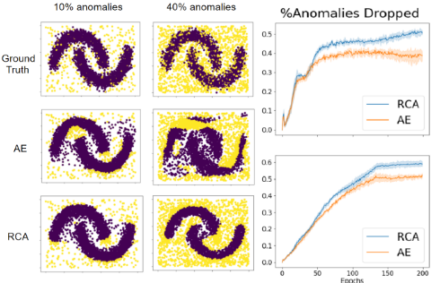
To understand how RCA overcomes the limitations of conventional autoencoders (AE), we created a synthetic dataset containing a pair of crescent-shaped moons with Gaussian noise [Pedregosa et al., 2011] representing the normal observations and anomalies generated from a uniform distribution. In this experiment, we vary the proportion of anomalies from 10% to 40% while fixing the sample size to be 10,000. Samples with the top-[(1 - ϵ)n] highest anomaly scores are classified as anomalies, where ϵ is the anomaly ratio.
Figure 2 compares the performance of standard autoencoders (AE) against RCA for 10% (left column) and 40% (right column) anomaly ratio. Although the performance for both methods degrades with increasing anomaly ratio, RCA is more robust compared to AE. In particular, when the anomaly ratio is 40%, AE fails to capture the true manifold of the normal data, unlike RCA. This result is consistent with the assertion in Theorem 2, which states that training the autoencoder with a subset of points selected by RCA is better than using all the data when anomaly ratio is large.
4.2 Results on Real-World Data
For evaluation, we used 18 benchmark datasets obtained from the Stony Brook ODDS library [Rayana, 2016] 1 . We reserve 60% of the data for training and the remaining 40% for testing. The performance of the competing methods are evaluated based on their Area under ROC curve (AUC) scores.
Baseline Methods We compared RCA against the following baseline methods: Deep-SVDD (deep one-class SVM) [Ruff et al., 2018], VAE (Variational autoencoder) [Kingma and Welling, 2013; An and Cho, 2015], DAGMM (deep gaussian mixture model) [Zong et al., 2018], SO-GAAL (Single-Objective Generative Adversarial Active Learning) [Liu et al., 2019], OCSVM (one-class SVM) [Chen et al., 2001], and IF (isolation forest) [Liu et al.,
1 Additional experimental results on the CIFAR10 dataset are given in the longer version of the paper.
| RCA | VAE | AE | SO GAAL | DAGMM | Deep-SVDD | OCSVM | IF | |
|---|---|---|---|---|---|---|---|---|
| vowels | 0.917±0.016 | 0.503±0.045 | 0.879±0.020 | 0.637±0.197 | 0.340±0.103 | 0.206±0.035 | 0.765±0.036 | 0.768±0.013 |
| pima | 0.711±0.016 | 0.648±0.015 | 0.669±0.013 | 0.613±0.049 | 0.531±0.025 | 0.395±0.034 | 0.594±0.026 | 0.662±0.018 |
| optdigits | 0.890±0.041 | 0.909±0.016 | 0.907±0.010 | 0.487±0.138 | 0.290±0.042 | 0.506±0.024 | 0.558±0.009 | 0.710±0.041 |
| sensor | 0.950±0.030 | 0.913±0.003 | 0.866±0.050 | 0.557±0.224 | 0.924±0.085 | 0.614±0.073 | 0.939±0.002 | 0.948±0.002 |
| letter | 0.802±0.036 | 0.521±0.042 | 0.829±0.031 | 0.601±0.060 | 0.433±0.034 | 0.465±0.039 | 0.557±0.038 | 0.643±0.040 |
| cardio | 0.905±0.012 | 0.944±0.006 | 0.867±0.020 | 0.473±0.075 | 0.862±0.031 | 0.505±0.056 | 0.936±0.002 | 0.927±0.006 |
| arrhythmia | 0.806±0.044 | 0.811±0.034 | 0.802±0.044 | 0.538±0.042 | 0.603±0.095 | 0.635±0.063 | 0.782±0.028 | 0.802±0.024 |
| breastw | 0.978±0.003 | 0.950±0.006 | 0.973±0.004 | 0.980±0.011 | 0.976±0.000 | 0.406±0.037 | 0.955±0.006 | 0.983±0.008 |
| musk | 1.000±0.000 | 0.994±0.002 | 0.998±0.003 | 0.234±0.193 | 0.903±0.130 | 0.829±0.048 | 1.000±0.000 | 0.995±0.006 |
| mnist | 0.858±0.012 | 0.778±0.009 | 0.802±0.009 | 0.795±0.025 | 0.652±0.077 | 0.538±0.048 | 0.835±0.012 | 0.800±0.013 |
| satimage-2 | 0.977±0.008 | 0.966±0.008 | 0.818±0.069 | 0.789±0.177 | 0.853±0.113 | 0.739±0.088 | 0.998±0.003 | 0.996±0.004 |
| satellite | 0.712±0.011 | 0.538±0.016 | 0.575±0.068 | 0.640±0.070 | 0.667±0.189 | 0.631±0.016 | 0.650±0.014 | 0.700±0.031 |
| mammogr. | 0.844±0.014 | 0.864±0.014 | 0.853±0.015 | 0.204±0.026 | 0.834±0.000 | 0.272±0.009 | 0.881±0.015 | 0.873±0.021 |
| thyroid | 0.956±0.008 | 0.839±0.011 | 0.928±0.020 | 0.984±0.005 | 0.582±0.095 | 0.704±0.027 | 0.960±0.006 | 0.980±0.006 |
| annthyroid | 0.688±0.016 | 0.589±0.021 | 0.675±0.022 | 0.679±0.022 | 0.506±0.020 | 0.591±0.014 | 0.599±0.013 | 0.824±0.009 |
| ionosphere | 0.846±0.015 | 0.763±0.015 | 0.821±0.010 | 0.783±0.080 | 0.467±0.082 | 0.735±0.053 | 0.812±0.039 | 0.843±0.020 |
| pendigits | 0.856±0.011 | 0.931±0.006 | 0.685±0.073 | 0.257±0.053 | 0.872±0.068 | 0.613±0.071 | 0.935±0.003 | 0.941±0.009 |
| shuttle | 0.935±0.013 | 0.987±0.001 | 0.921±0.013 | 0.571±0.316 | 0.890±0.109 | 0.531±0.290 | 0.985±0.001 | 0.997±0.001 |
2008]. Note that Deep-SVDD and DAGMM are two recent deep AD methods while OCSVM and IF are state-of-the-art unsupervised AD methods. In addition, we also perform an ablation study to compare RCA against its four variants: AE (standard autoencoders without collaborative networks) and RCA-E (RCA without ensemble evaluation), and RCA-SS (RCA without sample selection). To ensure fair comparison, we maintain similar hyperparameter settings for all the competing DNN-based approaches. Experimental results are reported based on their average AUC scores across 10 random initializations. More discussion about our experimental setting will be given in the long version of the paper.
Performance Comparison The results summarized in Table 1 show that RCA outperforms all the deep unsupervised AD methods (SO-GAAL, DAGMM, Deep-SVDD) in 16 out of 18 datasets. RCA also performs better than both AE and VAE in 11 out of the 18 datasets, IF in 10 of the datasets, and OCSVM in 11 of the datasets. These results suggest that RCA clearly outperforms the baseline methods on majority of the datasets. Surprisingly, some of the complex DNN baselines such as SO-GAAL, DAGMM, and Deep-SVDD perform poorly on the datasets. This is because most of these DNN methods assume the availability of clean training data, whereas in our experiments, the training data are contaminated with anomalies to reflect a more realistic setting. Furthermore, we use the same network architecture for all the DNN methods (including RCA), since there is no guidance on how to best tune the network structure given that it is an unsupervised AD task.
RCA for Missing Values As real-world data are imperfect, we compare the performance of RCA and other baseline methods in terms of their robustness to missing values. Mean imputation is a common approach to deal with missing values. In this experiment, we add missing values randomly in the features of each benchmark dataset and apply mean imputation to replace the missing values. Such imputation will likely introduce noise into the data. We vary the percentage of missing values from 10% to 50% and compare the average AUC scores of the competing methods. The number of wins, draws, and losses of RCA compared to each baseline method on the 18 benchmark datasets is given in Table 2. RCA was found to consistently outperform both DAGMM and DeepSVDD by more than 80%, demonstrating its robustness compared to other deep unsupervised AD methods when training data is contaminated. Additionally, as the missing ratio increases to more than 30%, it outperforms IF and OCSVM on more than 70% on the datasets. The results suggest that our framework is better than the baselines on the majority of the datasets in almost all settings.
Ablation Study We have also performed an ablation study to investigate the effectiveness of using sample selection and ensemble evaluation. The results comparing RCA against its variants, RCA-E, RCA-SS, and AE are given in Table 2. Without missing value imputation, RCA outperformed all the variants in at least 11 of the datasets. The advantage of RCA over its variants, AE, RCA-SS, and RCA-E, reduces with increasing amount of noise due to missing value imputation but is still significant until the missing ratio is 50%.
Sensitivity Analysis RCA requires users to specify the anomaly ratio of the data. Since the true anomaly ratio ϵ is often unknown, we conducted experiments to evaluate the robustness of RCA when ϵ is overestimated or underestimated by 5% and 10%. from their true values on all datasets. The results in Table 3 suggest that the AUC scores for RCA do not change significantly even when the anomaly ratio was overestimated or underestimated by 10% on most of the datasets.
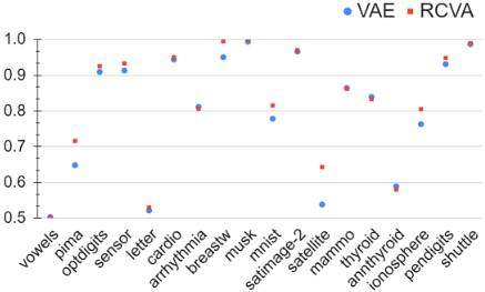
RCA with VAE The results reported for RCA in Tables 1 - 3 use autoencoders as the underlying DNN. To investigate whether our framework can benefit other DNN architectures, we compared our Robust Collaborative Variational Autoencoder (RCVA) against traditional VAE. The results in Figure 3 showed that RCVA outperformed VAE on most of the datasets, which suggests that our framework can improve the performance of VAE for unsupervised AD.
| Missing Ratio | RCA-E | RCA-SS | VAE | SO- GAAL | AE | DAGMM | Deep- SVDD | OCSVM | IF |
|---|---|---|---|---|---|---|---|---|---|
| 0.0 | 11-2-5 | 16-0-2 | 12-0-6 | 16-0-2 | 15-0-3 | 17-0-1 | 18-0-0 | 11-1-6 | 10-0-8 |
| 0.1 | 12-1-5 | 14-1-3 | 16-1-1 | 16-0-2 | 14-0-4 | 17-0-1 | 18-0-0 | 13-1-4 | 12-0-6 |
| 0.2 | 11-1-6 | 13-3-2 | 14-2-2 | 17-0-1 | 13-0-5 | 18-0-0 | 18-0-0 | 15-0-3 | 9-0-9 |
| 0.3 | 9-3-6 | 13-1-4 | 15-0-3 | 17-1-0 | 13-0-5 | 18-0-0 | 18-0-0 | 16-0-2 | 14-1-3 |
| 0.4 | 10-0-8 | 12-2-4 | 14-0-4 | 15-0-3 | 12-0-6 | 17-0-1 | 18-0-0 | 16-0-2 | 15-0-3 |
| 0.5 | 8-3-7 | 10-1-7 | 11-1-6 | 14-0-4 | 9-0-9 | 15-0-3 | 17-0-1 | 14-1-3 | 13-0-5 |
| Perturbed anomaly ratio, ∆ϵ | ||||
|---|---|---|---|---|
| Dataset | -0.1 | -0.05 | 0.05 | 0.1 |
| vowels | 0.908 | 0.908 | 0.918 | 0.920 |
| pima | 0.697 | 0.704 | 0.719 | 0.721 |
| optdigits | 0.861 | 0.861 | 0.973 | 0.980 |
| sensor | 0.913 | 0.913 | 0.876 | 0.876 |
| letter | 0.802 | 0.802 | 0.793 | 0.796 |
| cardio | 0.851 | 0.860 | 0.923 | 0.947 |
| arrhythmia | 0.806 | 0.806 | 0.807 | 0.807 |
| breastw | 0.970 | 0.973 | 0.981 | 0.983 |
| musk | 0.809 | 0.809 | 1.000 | 1.000 |
| mnist | 0.847 | 0.851 | 0.852 | 0.840 |
| satimage-2 | 0.965 | 0.965 | 0.998 | 0.998 |
| satellite | 0.713 | 0.718 | 0.701 | 0.688 |
| mammography | 0.838 | 0.838 | 0.854 | 0.840 |
| thyroid | 0.949 | 0.949 | 0.959 | 0.957 |
| annthyroid | 0.669 | 0.683 | 0.693 | 0.689 |
| ionosphere | 0.862 | 0.855 | 0.844 | 0.841 |
| pendigits | 0.858 | 0.858 | 0.858 | 0.847 |
| shuttle | 0.958 | 0.956 | 0.949 | 0.994 |
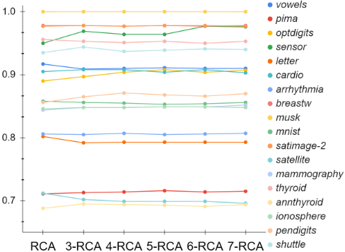
RCA with Multiple Networks To extend RCA from 2 to multiple DNNs, we modified the shuffling step to allow each DNN to shuffle its selected data to any of the other DNNs. We varied the number of DNNs from 2 to 7 and plotted the results in Figure 4. The results suggest that adding more DNNs does not help significantly. This is not surprising since the shuffling step is designed to prevent the DNNs from converging too quickly rather than as an ensemble framework to boost performance. Increasing the number of DNNs also makes it more expensive to train, which reduces its benefits.
5 Conclusion
This paper introduces RCA framework for unsupervised AD to overcome limitations of existing DNN methods. Theoretical analysis shows the effectiveness of RCA in eliminating corruption in training data. Our results showed that RCA outperforms various algorithms under different experimental settings and is robust to missing value.
Acknowledgements
This research was supported in part by the grant National Science Foundation IIS-2006633, EF-1638679, IIS-1749940, Office of Naval Research N00014-20-1-2382, National Institute on Aging RF1AG072449. Any use of trade, firm or product names is for descriptive purposes only and does not imply endorsement by the U.S. Government.
@inproceedings{ijcai2021p208,
  title     = {RCA: A Deep Collaborative Autoencoder Approach for Anomaly Detection},
  author    = {Liu, Boyang and Wang, Ding and Lin, Kaixiang and Tan, Pang-Ning and Zhou, Jiayu},
  booktitle = {Proceedings of the Thirtieth International Joint Conference on
               Artificial Intelligence, {IJCAI-21}},
  publisher = {International Joint Conferences on Artificial Intelligence Organization},
  editor    = {Zhi-Hua Zhou},
  pages     = {1505--1511},
  year      = {2021},
  month     = {8},
  note      = {Main Track},
  doi       = {10.24963/ijcai.2021/208},
  url       = {https://doi.org/10.24963/ijcai.2021/208},
}
TY - CPAPER TI - RCA: A Deep Collaborative Autoencoder Approach for Anomaly Detection AU - Liu, Boyang AU - Wang, Ding AU - Lin, Kaixiang AU - Tan, Pang-Ning AU - Zhou, Jiayu T2 - Proceedings of the Thirtieth International Joint Conference on Artificial Intelligence, IJCAI-21 PB - International Joint Conferences on Artificial Intelligence Organization PY - 2021 SP - 1505 EP - 1511 DO - 10.24963/ijcai.2021/208 UR - https://doi.org/10.24963/ijcai.2021/208 ER -Copied
Machine-readable versions of this paper, for tools and AI agents:





